

Mathematical Foundations of Contrastive Loss
Introduction to Contrastive Learning
For a classical problem like vector clustering or image classification, Cross-Entropy turns out to be a popularly used loss function. Here, the model learns by directly comparing its predicted output with the ground-truth labels, aiming for a minimum difference between them.
However, we can take this a step further by not only pulling predictions toward the correct labels, but also pushing them away from incorrect ones.
For instance, tigers and dogs look very similar (ok maybe different for humans but), so the embedding model could place them close together in vector space. However, since they are in different classes, the model is trained such that tiger vectors should be close to other tiger vectors, dog vectors should be close to other dog vectors, and tiger and dog vectors should be far apart.
As a result, the model learns to maximize similarity with positive targets (correct labels) while minimizing similarity with negative targets (incorrect labels).
Triplet Loss
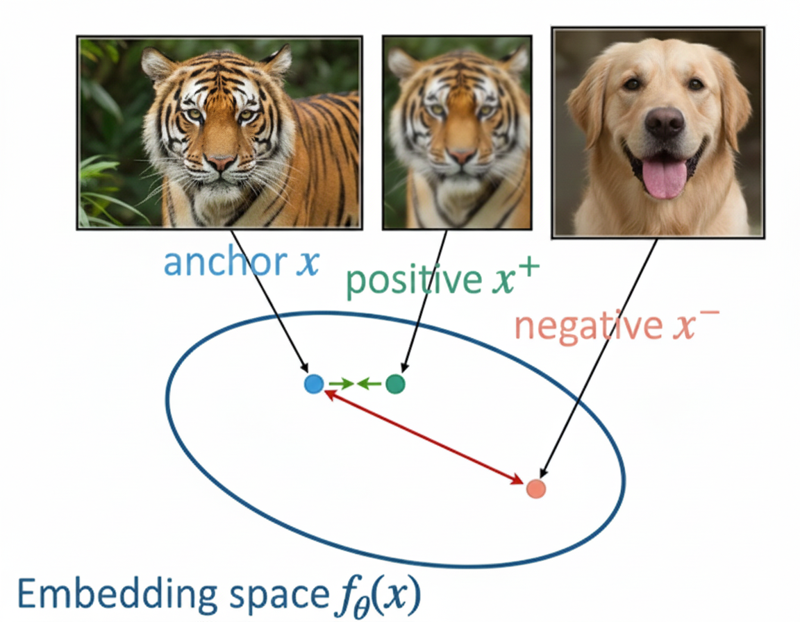
Triplet loss is one of the early contrastive loss which was introduced in the 2015 paper “FaceNet: A Unified Embedding for Face Recognition and Clustering”. In this work, the authors proposed triplets of samples (anchor, positive, negative) to train an embedding model.
The anchor is a selected sample (e.g., an image of a tiger), positive is a different sample from the same class (e.g an image of another tiger), and negative is a sample from a different class (e.g., an image of a dog). So basically Triplet loss objective is “Anchor should be closer to Postive than to Negative”
Note: In practice, the positive sample is an augmented version of the anchor (done by different techniques like Random rotation, Crop, etc), this is case used for self-supervised where labels are not known.
Mathematically, the triplet loss is defined as:
\[L = \min_{\theta} \sum_{i=1}^{N} \max\left( \| f_{\theta}(x_i^{a}) - f_{\theta}(x_i^{p}) \|_2^2 - \| f_{\theta}(x_i^{a}) - f_{\theta}(x_i^{n}) \|_2^2 + \alpha, 0 \right)\](Schroff et al., 2015)
Here, $x_i^{a}$, $x_i^{p}$, and $x_i^{n}$ represent the anchor, positive, and negative samples, respectively. The embedding function $f_{\theta}(\cdot)$, parameterized by $\theta$, maps inputs to a embedding space, while the margin $\alpha$ enforces a minimum separation between the anchor–positive and anchor–negative distances, ensuring that the negative sample is at least $\alpha$ farther away from the anchor than the positive sample. If this condition is already satisfied, the loss for that triplet becomes zero.
InfoNCE
InfoNCE is similar to triplet loss, but it addresses an important limitation: what if there are many negative examples instead of just one?
Triplet loss compares an anchor with one positive and one negative sample at a time. InfoNCE is an extension of this by allowing the anchor to be compared against multiple negative samples at once.
First, the model computes similarity scores between the anchor and one positive sample, as well as between the anchor and many negative samples. These similarity scores are then passed through a softmax function, which converts them into probabilities that sum to one.
The training objective is to assign high similarity score to positive sample and lower to negative samples.
Mathematically, the InfoNCE loss is defined as:
\[L = - \log \frac{ \exp(s^{+}/\tau) }{ \exp(s^{+}/\tau) + \sum_{i=1}^{N-1} \exp(s_i^{-}/\tau) }\](van den Oord et al., 2018)
In this objective, $s^{+}$ is the similarity between the anchor and the positive sample, while $s_i^{-}$ measures the similarity between the anchor and each of the $N-1$ negative samples.
The relationship between these values is modulated by $\tau$, a temperature scaling factor. By adjusting $\tau$, we can dictate how aggressively the model penalizes “hard negatives”; those samples that are mathematically similar to the anchor despite being distinct.
Note: Triplet loss was originally supervised but can be adapted for self-supervised learning. InfoNCE is a contrastive loss specifically designed for self-supervised representation learning.
Proof: InfoNCE as Categorical Cross-Entropy
The goal is to show that the InfoNCE loss can be interpreted as a categorical cross-entropy (CCE) loss over multiple classes,
The standard categorical cross-entropy loss for $C$ classes is defined as:
\[\mathcal{L}_{CCE} = -\sum_{j=1}^{C} y_j \log(\hat{\rho}_j)\]Where, $y_j$ represents the one-hot target vector, which indicates the ground-truth label, while $\hat{\rho}_j$ denotes the model’s predicted probability for class $j$.
In this scenario, the positive pair represents the only “correct” class ($y=1$), while all $N-1$ negative pairs are treated as “incorrect” ($y=0$).
\[\mathcal{L}_{CCE} = -\left(1 \cdot \log(\hat{\rho}_{\text{pos}}) + \sum_{j=1}^{N-1} 0 \cdot \log(\hat{\rho}_{\text{neg}, j})\right)\]the formula simplifies significantly.
\[\mathcal{L} = -\log(\hat{\rho}_{\text{pos}})\]In this setup, the probability assigned to the positive pair is calculated by applying a softmax over the similarity scores.
\[\hat{\rho}_{\text{pos}} = \frac{ \exp(s^{+}/\tau) }{ \exp(s^{+}/\tau) + \sum_{i=1}^{N-1} \exp(s_i^{-}/\tau) }\]When we substitute the softmax probability into our cross-entropy expression, we arrive at the InfoNCE (Information Noise-Contrastive Estimation) loss for a single sample.
\[\mathcal{L} = - \log \left( \frac{ \exp(s^{+}/\tau) }{ \exp(s^{+}/\tau) + \sum_{i=1}^{N-1} \exp(s_i^{-}/\tau) } \right)\]To train the model effectively, we don’t just look at one example at a time. Instead, we calculate the Total Loss across a batch of $N$ anchors, taking the average to ensure stable gradients.
\[\mathcal{L}_{\text{total}} = \frac{1}{N} \sum_{i=1}^{N} - \log \frac{ \exp(s_i^{+}/\tau) }{ \exp(s_i^{+}/\tau) + \sum_{j=1}^{N-1} \exp(s_{i,j}^{-}/\tau) }\]To view the objective from a broader, more theoretical lens, we can express the loss as an expectation over the entire data distribution.
\[\mathcal{L}_{\text{InfoNCE}} = - \mathbb{E}_{(x, x^+)\sim p_\text{data}} \Bigg[ \log \frac{ \exp(s(x, x^+)/\tau) }{ \exp(s(x, x^+)/\tau) + \sum_{x^- \sim p_\text{neg}} \exp(s(x, x^-)/\tau) } \Bigg]\]Visualization of Loss Function
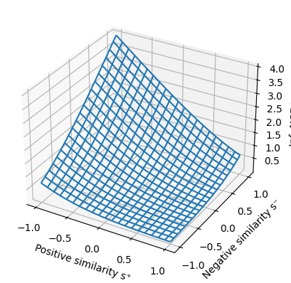
We can visualize the InfoNCE loss as a 3D plot. The axes represent positive similarity ($s^{+}$) and negative similarity ($s^{-}$), with the height of the surface representing the loss value. This surface slopes downward toward a “sweet spot” where $s^{+}=1$ and $s^{-}=-1$.
At this ideal point, the loss reaches zero, indicating the model has perfectly learned to pull similar pairs together and push dissimilar ones apart.
InfoNCE: A Lower Bound on Mutual Information
Prerequisite: Basics on Mutal Information
Here we will connect InfoNCE with Information Theory. Below is the proof on how minimizing this loss maximizes a lower bound on the Mutual Information.
Given the InfoNCE loss for a single anchor:
\[L = -\mathbb{E} \log \frac{\exp(s^+ / \tau)}{\exp(s^+ / \tau) + \sum_{i=1}^{N-1} \exp(s^-_i / \tau)}\]If we assume an optimal similarity function $s^*(x, x’)$, we can define it as (see Optimal Bayes’s theorem for more detail):
\[s^*(x, x') = \tau \log \frac{p(x, x')}{p(x)p(x')}\] \[\implies \exp(s^*/\tau) = \frac{p(x, x')}{p(x)p(x')}\]Substituting this optimal similarity into the loss function $L^{opt}_N$:
\[L^{opt}_N = -\mathbb{E} \log \frac{\frac{p(x,x^+)}{p(x)p(x^+)}}{\frac{p(x,x^+)}{p(x)p(x^+)} + \sum_{i=1}^{N-1} \frac{p(x,x^-_i)}{p(x)p(x^-_i)}}\]By approximating the sum in the denominator and simplifying the expression, we arrive at:
\[\approx \mathbb{E} \log \left[ 1 + N \frac{p(x)p(x^+)}{p(x,x^+)} \right]\]This leads to the bound:
\[L^{opt}_N \geq \log N - \mathbb{E} \log \frac{p(x,x^+)}{p(x)p(x^+)}\]Since the second term on the right is the definition of Mutual Information $I(X; X^+)$, we can rearrange the inequality to show:
\[I(X; X^+) \geq \log N - L^{opt}_N\]This proof, popularized by van den Oord et al. (2018), demonstrates that as we increase the number of negative samples $N$ and decrease the loss $L$, we effectively force the model to capture more shared information between the anchor and the positive sample.
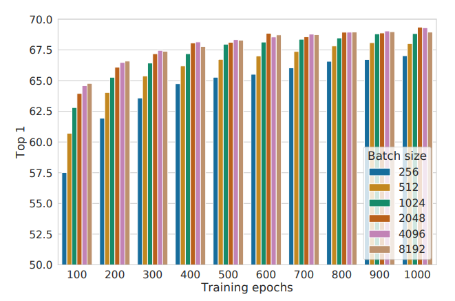
The Necessity of Large Batch Sizes
The relationship between mutual information and InfoNCE reveals a fundamental constraint known as the Mutual Information Ceiling.
According to the inequality $I(X; X^+) \geq \log N - L^{\text{opt}}_N$, This means the maximum information the model can learn is limited by $\log N$, so the learning capacity is capped by the number of negative samples 𝑁, This is clearly seen in models like SimCLR which scales so effectively with increase in batch sizes.
Question:
If InfoNCE considers only the augmented sample x⁺ as positive and treats all other samples; including other positives of the same class as negatives, how does the model still learn meaningful representations?
Answer
The model still learns because even if it pushes away treating same-class as negative, it’s simultaneously pulled toward its positive pair, so similar samples naturally cluster together over time. Also, in large dataset the occurence of same pair is very low in sample batch size.Supervised Contrastive Loss (SupCon)
In the figure below, self supervised learning using InfoNCE treats only the augmented version of an image as a positive, while all other images, even those showing dogs, are treated as negatives. In contrast, supervised contrastive learning uses labels so all dog images are treated as positives and are pulled closer together.
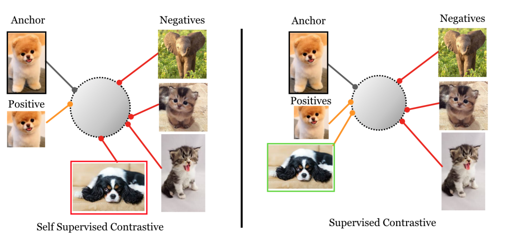
Therefore, instead of treating only an augmented view of the same sample as positive, all samples that share the same class label as the anchor are considered positives.
For a given anchor $i$, let $P(i)$ be the set of indices for all other samples in the batch sharing the same label, and let $A(i)$ represent all indices in the batch excluding the anchor itself. The loss is defined as:
\[L_{\text{sup}} = \sum_{i \in I} \frac{-1}{|P(i)|} \sum_{p \in P(i)} \log \frac{\exp(z_i \cdot z_p / \tau)}{\sum_{a \in A(i)} \exp(z_i \cdot z_a / \tau)}\](Khosla et al., 2020)
SupCon pulls all samples from the same class together while simultaneously pushing away samples from different classes.
Toy Numerical Example
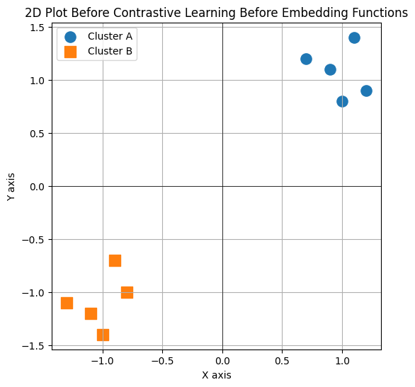
This given data sets looks like:
$A=(1.0, 0.8), (0.7, 1.2), (1.1, 1.4), (0.9, 1.1), (1.2, 0.9)$
$B = {(- 1.1, -1.2), (-0.8, -1.0), (-1.3, -1.1), (-0.9, -0.7), (-1.0, -1.4)}$
Now if we apply supervised contrastive loss for the above data,
We start with anchor $a1$. In our batch, we have four positive matches ($a2$ through $a5$) and five negatives ($b1$ to $b5$). Using a temperature of $\tau = 0.1$ sharpens the focus, making the model more sensitive to small differences in similarity.
Pairwise Similarity Computation:
| Pair ($a1, \cdot$) | cos | cos / $\tau$ | exp($\cdot$) |
|---|---|---|---|
| $a2$ | 0.92 | 9.2 | $9.9 \times 10^3$ |
| $a3$ | 0.95 | 9.5 | $1.33 \times 10^4$ |
| $a4$ | 0.98 | 9.8 | $1.80 \times 10^4$ |
| $a5$ | 0.96 | 9.6 | $1.48 \times 10^4$ |
| $b1$-$b5$ | $\approx -0.95$ | $\approx -9.5$ | $\approx 0$ |
Denominator (total sum): $\sum_{k \neq a1} \exp(s_{1k}) = 9,900 + 13,300 + 18,000 + 14,800 + negatives = \mathbf{56,000}$
we take the log of each positive’s score divided by the total sum ( Log-Probability Terms (Positive Pairs)):
| Positive Pair ($a1, p$) | $\log \frac{\exp(s_{1p})}{\sum_{k \neq a1} \exp(s_{1k})}$ |
|---|---|
| $a2$ | -1.73 |
| $a3$ | -1.44 |
| $a4$ | -1.13 |
| $a5$ | -1.32 |
To get the specific loss for anchor $a1$, we simply average those four log-probability terms and flip the sign:
\[L_{a1} = -\frac{1}{|P(a1)|} \sum_{p \in P(a1)} \log \frac{\exp(s_{1p})}{\sum_{k \neq a1} \exp(s_{1k})}\] \[= -\frac{1}{4} \sum_{p \in \{a2, a3, a4, a5\}} \log \frac{\exp(s_{1p})}{\sum_{k \neq a1} \exp(s_{1k})} \approx 1.40\]If this were a full training step with 10 different anchors, we would repeat this for each one ($L_{a2}, L_{a3} \dots$) and take the average of all ten to get our final $L_{\text{total}}$
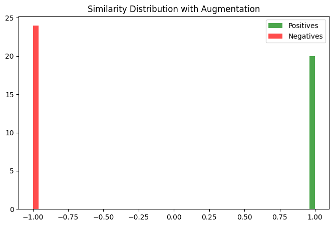
Histrogram Plot of Similarites After Training
The histogram shows the distribution of similarity scores (Cosine) for positive and negative pairs in the embedding space after training using supervised Contrastive loss (SupCon). This separation reflects the effectiveness of contrastive learning in creating a discriminative embedding space.
Conclusion
The key takeaway is that contrastive learning is not just a method for classification, it can be applied across a wide spectrum of tasks, including NLP, computer vision, and more. As seen above, it can be used with both labeled (SupCon) and unlabeled data (InfoNCE).
The objective of this loss function is to mimic human thinking: distinguishing how similar items are to each other while recognizing how dissimilar they are from others.
This article has introduced you to the world of contrastive learning, with much more to explore.
“The world is your oyster”, Thank you.
References
-
Florian Schroff, Dmitry Kalenichenko, and James Philbin. “FaceNet: A Unified Embedding for Face Recognition and Clustering”. 2015 IEEE Conference on Computer Vision and Pattern Recognition (CVPR), 2015. doi: 10.1109/cvpr.2015.7298682
-
Aaron van den Oord, Yazhe Li, and Oriol Vinyals. “Representation Learning with Contrastive Predictive Coding”. arXiv:1807.03748 (2018). doi: 10.48550/arxiv.1807.03748
-
Ting Chen, Simon Kornblith, Mohammad Norouzi, and Geoffrey Hinton. “A Simple Framework for Contrastive Learning of Visual Representations”. arXiv:2002.05709 (2020). doi: 10.48550/arxiv.2002.05709
-
Prannay Khosla et al. “Supervised Contrastive Learning”. arXiv:2004.11362 (2021). doi: 10.48550/arxiv.2004.11362