
Introduction to Autoencoder
Autoencoder
Difference between generative and discriminative modelling
Generative modelling
Generative modelling is a statistical modeling technique that aims to model the entire probability distribution of the data. In other words, it tries to model the underlying patterns and relationships that generate the observed data. Given a set of inputs, a generative model generates new examples that are similar to the training data. Generative models are trained to learn the joint probability distribution $P(X,Y)$ of the input $X$ and the output $Y$.
Some examples of generative models include Gaussian mixture models, Hidden Markov Models, and Variational Autoencoders.
Discriminative modelling
Discriminative modelling, on the other hand, focuses on modeling the conditional probability distribution $P(Y, X)$, which is the probability of the output $Y$ given the input $X$. Discriminative models try to learn the decision boundary that separates different classes in the data. Discriminative models are trained to learn the mapping function from input X to output $Y$.
Some examples of discriminative models include Logistic Regression, Support Vector Machines, and Neural Networks.
Motivation behind Autoencoders
The main motivation behind Autoencoders is to learn an efficient data representation or encoding of the input data, which can be used for tasks such as data compression, denoising, feature extraction, and data generation. Autoencoders are a type of neural network that consists of an encoder and a decoder, which are trained together to learn a compressed representation of the input data.
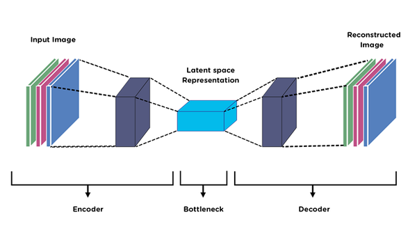
The basic idea of an autoencoder is to compress the input data into a lower-dimensional representation and then reconstruct the original data from this compressed representation. The encoder maps the input data to a lower-dimensional latent space, while the decoder maps the latent space back to the original data space. The goal of training the autoencoder is to minimize the difference between the input data and the reconstructed output data, which is typically measured using a loss function such as mean squared error.
Here is an example of an autoencoder architecture:

One of the main advantages of using autoencoders is that they can learn representations of the data that are robust to noise and can capture the underlying structure of the data. Autoencoders have been successfully used in a variety of applications, including image and speech recognition, anomaly detection, and natural language processing.
Basic structure of Autoencoder
Autoencoders are a type of neural network that can be used to learn a compressed representation of input data, such as images. The basic structure of an autoencoder with images typically consists of two main parts: an encoder and a decoder.
The encoder takes an input image and compresses it into a lower-dimensional latent representation, also known as the encoding. The encoder can consist of several layers of convolutional or pooling operations followed by fully connected layers, which map the input image to a lower-dimensional vector representation.
class Encoder(nn.Module):
    def __init__(self, channels, embedding_dim):
        super(Encoder, self).__init__()
        self.conv1 = nn.Conv2d(channels, 32, kernel_size=3, stride=2, padding=1)
        self.conv2 = nn.Conv2d(32, 64, kernel_size=3, stride=2, padding=1)
        self.conv3 = nn.Conv2d(64, 128, kernel_size=3, stride=2, padding=1)
        self.flatten = nn.Flatten()
        self.fc = nn.Linear(128 * 4 * 4, embedding_dim)

    def forward(self, x):
        x = self.conv1(x)
        x = nn.ReLU()(x)
        x = self.conv2(x)
        x = nn.ReLU()(x)
        x = self.conv3(x)
        x = nn.ReLU()(x)
        x = self.flatten(x)
        x = self.fc(x)
        return x
The decoder takes the encoding produced by the encoder and generates a reconstructed output image. The decoder can consist of several layers of convolutional or upsampling operations followed by fully connected layers, which map the latent representation back to the original image space.
class Decoder(nn.Module):
    def __init__(self, channels, embedding_dim):
        super(Decoder, self).__init__()
        self.fc = nn.Linear(embedding_dim, 128 * 4 * 4)
        self.unflatten = nn.Unflatten(1, (128, 4, 4))
        self.deconv1 = nn.ConvTranspose2d(128, 128, kernel_size=3, stride=2, padding=1, output_padding=1)
        self.deconv2 = nn.ConvTranspose2d(128, 64, kernel_size=3, stride=2, padding=1, output_padding=1)
        self.deconv3 = nn.ConvTranspose2d(64, 32, kernel_size=3, stride=2, padding=1, output_padding=1)
        self.output = nn.Conv2d(32, channels, kernel_size=1, stride=1)

    def forward(self, x):
        x = self.fc(x)
        # x = x.reshape(x.shape[0], 128, 4, 4)
        x = self.unflatten(x)
        x = self.deconv1(x)
        x = nn.ReLU()(x)
        x = self.deconv2(x)
        x = nn.ReLU()(x)
        x = self.deconv3(x)
        x = nn.ReLU()(x)
        x = self.output(x)
        return x
The encoder and decoder are trained together to minimize the difference between the input image and the reconstructed output image using a loss function such as mean squared error. During training, the encoder learns to capture the essential features of the input image in the latent representation, while the decoder learns to reconstruct the image from the latent representation.
class Autoencoder(nn.Module):
    def __init__(self, channels, embedding_dim):
        super(Autoencoder, self).__init__()
        self.encoder = Encoder(channels, embedding_dim)
        self.decoder = Decoder(channels, embedding_dim)

    def forward(self, x):
        x = self.encoder(x)
        x = self.decoder(x)
        return x
The architecture of an autoencoder can vary depending on the specific application and the characteristics of the input data. For example, variations of autoencoders such as denoising autoencoders, variational autoencoders, and adversarial autoencoders can be used for specific tasks and to overcome certain limitations of traditional autoencoders.
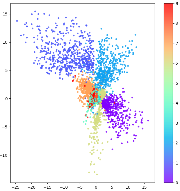
Visualization of Results from Autoencoder on MNIST dataset
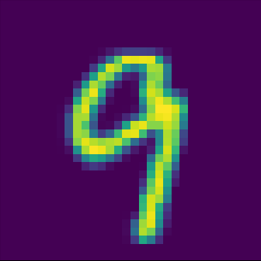
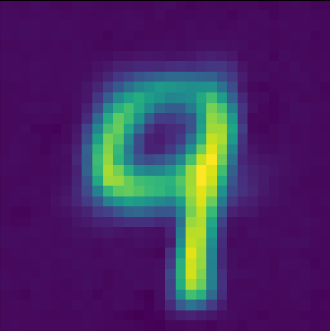
While learning the representation of MNIST dataset on a low dimensional latent space. we can force that dimension to be 2D and visualize the representation of numbers in their repective clusters.
Autoencoder vs PCA vs SVD
Autoencoder, Principal Component Analysis (PCA), and Singular Value Decomposition (SVD) are all methods for reducing the dimensionality of data. However, there are several key differences between these methods.
Autoencoders are a type of neural network that can be used to learn a compressed representation of input data. Unlike PCA and SVD, autoencoders can learn non-linear relationships between the input data, which can make them more effective at capturing complex patterns and features in the data. Autoencoders are also capable of generating new data samples that are similar to the input data, which can be useful for tasks such as data augmentation and image generation.
PCA is a statistical technique that uses linear algebra to transform high-dimensional data into a lower-dimensional representation. PCA works by identifying the principal components of the data, which are the directions in the data that explain the most variance. These principal components can then be used to project the data onto a lower-dimensional subspace. PCA is a linear technique and can be limited in its ability to capture non-linear relationships between the input data.
SVD is a matrix factorization technique that can be used for dimensionality reduction. SVD works by decomposing a data matrix into three matrices, where the middle matrix represents the singular values of the data. The singular values can be used to select the most important components of the data, which can then be used for projection into a lower-dimensional subspace. SVD is a linear technique and can be limited in its ability to capture non-linear relationships between the input data.
Limitation of Autoencoder and Introduction to Variational Autoencoder
One of the limitations of a standard autoencoder is that it does not have a probabilistic interpretation, which can make it difficult to generate new data samples or to perform tasks such as anomaly detection. The output of a standard autoencoder is a deterministic reconstruction of the input data, which may not accurately capture the variability in the data.
To address this limitation, Variational Autoencoder (VAE) was introduced, which is a type of generative model that has a probabilistic interpretation. VAE is also based on neural networks and consists of two main parts: an encoder and a decoder, similar to a standard autoencoder.
However, instead of directly learning the encoding of input data, VAE learns a probability distribution over the encoding. Specifically, VAE learns to map the input data to a mean and variance vector, which is then used to sample from a distribution. The sampled vector is then fed into the decoder to generate a reconstructed output.
The advantage of using a probabilistic framework is that it allows the generation of new data samples by randomly sampling from the learned distribution over the encoding space. This means that VAE can learn a richer representation of the input data and generate new samples that are similar to the training data but not necessarily identical.
One of the key differences between VAE and a standard autoencoder is the use of a loss function that incorporates both the reconstruction error and a regularization term. The regularization term ensures that the learned distribution over the encoding space follows a predefined distribution, such as a Gaussian distribution. This helps to prevent overfitting and encourages the model to learn a smooth and continuous representation of the data.
Conclusion
In all, Autoencoder is a powerful neural network architecture that has a wide range of applications in data compression, feature extraction, and data generation. It can learn a compressed representation of the input data that can be used for various downstream tasks. However, autoencoder has some limitations, such as its inability to model the probabilistic nature of data and its tendency to reconstruct the input data without capturing the variability in the data. Nonetheless, researchers have developed various variants of autoencoder, such as Variational Autoencoder (VAE) and Convolutional Autoencoder (CAE), which have overcome some of these limitations and have shown promising results in various fields.
References
[1] A Simple AutoEncoder and Latent Space Visualization with PyTorch
[2] Difference between AutoEncoder (AE) and Variational AutoEncoder (VAE)