Stochastic Gradient Descent: Theory, Numerical Examples, and Implementation

February 13, 2026 36 minute read

Introduction

Welcome to this comprehensive guide on Stochastic Gradient Descent (SGD), one of the most fundamental optimization algorithms in machine learning. This document provides a complete exploration of SGD from theoretical foundations to practical implementation, featuring detailed mathematical explanations, step-by-step numerical examples, and real-world coding applications.

Now that we’ve introduced the fundamental concepts of SGD, let’s dive deeper into the theoretical foundations that make this optimization algorithm mathematically sound and practically effective.

Gradient Descent vs Stochastic Gradient Descent

Feature	Gradient Descent (GD)	Stochastic Gradient Descent (SGD)
Scope	Uses ALL data points ($n$) for every step.	Uses ONE random data point (1) per step.
Mathematical Foundation	Calculates the True Gradient $ \nabla R(\theta) = \frac{1}{n}\sum \nabla \ell(\theta; x_i, y_i) $.	Calculates an Unbiased Estimate $ \nabla \ell(\theta; \xi) $ where $ \xi \sim D $.
Path Characteristics	Smooth, direct, and deterministic.	Noisy, zig-zag trajectory (High Variance).
Computational Cost	Very slow / Computationally expensive ($O(n)$).	Instant / Computationally cheap ($O(1)$).
Memory Requirements	Requires full dataset in memory.	Single sample at a time.
Convergence Properties	Guaranteed convergence to local/global minimum.	Converges in expectation with proper learning rate decay.
Analogy	“Walking with a complete GPS map.”	“Walking in the fog, seeing 1 step ahead.”

Mathematical Foundations

Expected Risk & Gradient Expectation (The Foundation)

Mathematical Statement:
The expected risk $R(\theta)$ is defined as the expected loss over the true data distribution $D$:

\[R(\theta) = \mathbb{E}[\ell(\theta; (x, y))] = \int \ell(\theta; (x, y)) \, dP(x, y)\]

The Unbiased Estimator Property:

\[\nabla R(\theta) = \mathbb{E}[\nabla \ell(\theta; \xi)] \quad \text{where } \xi \sim D\]

Proof Intuition:

The true gradient $ \nabla R(\theta) $ represents the gradient computed using the entire dataset
A single sample gradient $ \nabla \ell(\theta; \xi) $ is a random variable
When we average many single-sample gradients, we approach the true gradient
This is the mathematical foundation that makes SGD theoretically valid

Implications:

SGD is not “wrong” — it’s an unbiased estimator of the true gradient
Individual steps may be incorrect, but on average they point in the right direction
This property is essential for SGD’s mathematical legitimacy

Unbiasedness of Mini-Batch SGD (Real-World Application)

Mathematical Statement:
For a mini-batch $B$ of size $m$ with samples $ {\xi_1, \xi_2, \dots, \xi_m} $:

\[g(\theta) = \frac{1}{m} \sum_{i \in B} \nabla \ell(\theta; \xi_i)\] \[\mathbb{E}[g(\theta)] = \nabla R(\theta)\]

Proof:

$ \mathbb{E}[g(\theta)] = \mathbb{E}\left[\frac{1}{m} \sum_{i \in B} \nabla \ell(\theta; \xi_i)\right] $

$ = \frac{1}{m} \sum_{i \in B} \mathbb{E}[\nabla \ell(\theta; \xi_i)] \quad \text{(Linearity of expectation)} $

$ = \frac{1}{m} \sum_{i \in B} \nabla R(\theta) $

$ = \frac{1}{m} \cdot m \cdot \nabla R(\theta) $

$ = \nabla R(\theta) $

Practical Implications:

Mini-batching maintains the unbiased property while reducing variance
Larger batches provide more stable gradient estimates
Common batch sizes: 16, 32, 64, 128, 256, 512

Variance Scaling Analysis (The Problem)

Mathematical Statement:
The variance of the mini-batch gradient estimator scales with batch size:

\[\operatorname{Var}[g(\theta)] = \frac{1}{m} \cdot \sigma^2(\theta)\]

where $ \sigma^2(\theta) $ is the variance of individual sample gradients.

Key Insight:

Variance decreases linearly with batch size
To halve the variance, you need to double the batch size
To halve the standard deviation (noise), you need to quadruple the batch size
Even with large batches, variance never completely disappears

Mathematical Consequence:
With constant learning rate $ \eta $, SGD will oscillate around the minimum rather than converge exactly:

\[\limsup_{t \to \infty} \mathbb{E}\left[\lVert \theta_t - \theta^* \rVert^2\right] \ge C \cdot \eta\]

(for some constant $ C $)

Convergence Analysis: Robbins-Monro Conditions (The Solution)

The Challenge:
Due to persistent variance, constant learning rates cause SGD to oscillate around the minimum.

The Solution:
Use time-varying learning rates $ \eta_t $ that satisfy the Robbins–Monro conditions:

$ \sum_t \eta_t = \infty $ (Sum diverges — ensures progress toward minimum)
- This condition guarantees that the algorithm takes sufficiently large steps to reach the optimum
$ \sum_t \eta_t^2 < \infty $ (Sum of squares converges — ensures variance dies out)
- This condition ensures that the steps become small enough to prevent oscillation around the minimum

Common Learning Rate Schedules

Schedule Type	Formula	Description
Inverse decay	$ \eta_t = \frac{\eta_0}{1 + \lambda t} $	Learning rate decreases proportionally to inverse of iteration
Step decay	$ \eta_t = \eta_0 \times 0.1^{\lfloor t/T \rfloor} $	Learning rate drops by factor every $T$ epochs
Exponential decay	$ \eta_t = \eta_0 \times 0.95^t $	Learning rate decreases exponentially
Polynomial decay	$ \eta_t = \eta_0 \times t^{-\alpha}, \ \alpha \in (0.5, 1] $	Learning rate follows polynomial decay

Important Note on Exponential Decay

While exponential decay ($ \eta_t = \eta_0 \times 0.95^t $) does not strictly satisfy the Robbins–Monro conditions (since $ \sum_t \eta_t $ may converge for rapidly decaying rates), it is widely used in practice due to its effectiveness in achieving faster convergence during finite training periods. The practical benefits often outweigh the theoretical concerns in real-world applications.

Convergence Theorem

Under the Robbins–Monro conditions and appropriate smoothness assumptions:

\[\lim_{t \to \infty} \mathbb{E}\left[\lVert \nabla R(\theta_t) \rVert^2\right] = 0\]

meaning SGD converges to a stationary point in expectation.

The Complete Theoretical Framework

Component	Mathematical Statement	Purpose	Real-World Impact
Unbiasedness	$ \mathbb{E}[\nabla \ell(\theta; \xi)] = \nabla R(\theta) $	Validity foundation	SGD points in right direction on average
Mini-batch Scaling	$ \mathbb{E}[g(\theta)] = \nabla R(\theta) $	Practical efficiency	Enables batch processing
Variance Analysis	$ \operatorname{Var}[g(\theta)] = \frac{\sigma^2(\theta)}{m} $	Noise quantification	Explains zig-zag behavior
Convergence Conditions	$ \sum_t \eta_t = \infty,\ \sum_t \eta_t^2 < \infty $	Convergence guarantee	Learning rate decay rules

Numerical

Step-by-Step SGD Calculation Example

Let’s trace through a complete SGD iteration with logistic regression:

Model:

\[\hat{y} = \sigma(wx + b)\]

where

\[\sigma(z) = \frac{1}{1 + e^{-z}}\]

Loss (Binary Cross-Entropy):

\[L = -\left[y \log(\hat{y}) + (1-y)\log(1-\hat{y})\right]\]

Update Rule:

\[\theta \leftarrow \theta - \eta \nabla L\]

where $ \eta = 0.5 $ (learning rate).

Iteration	Sample Data (x,y)	Current $\theta[w,b]$	Logits $z$	Pred $\hat{y}$	Loss $L$	Gradient $\nabla[w,b]$	Updated $\theta[w,b]$
1	(3, 1)	[0, 0]	0	0.500	0.693	[-1.5000, -0.5000]	[0.750, 0.250]
2	(3, 0)	[0.7500, 0.2500]	2.5	0.924	2.577	[2.7723, 0.9241]	[-0.636, -0.212]
3	(1, 1)	[-0.6362, -0.2121]	-0.848	0.300	1.204	[-0.7002, -0.7002]	[-0.286, 0.138]

Detailed Calculation for Iteration 1
(x = 3, y = 1) with $\theta = [0, 0]$

1. Forward Pass

\[z = wx + b = 0 \times 3 + 0 = 0\] \[\hat{y} = \sigma(0) = \frac{1}{1 + e^{0}} = \frac{1}{2} = 0.5\]

2. Loss Calculation

\[L = -\left[1 \cdot \log(0.5) + 0 \cdot \log(0.5)\right] = -\log(0.5) = \ln(2) \approx 0.693\]

3. Gradient Computation

For logistic regression:

\[\nabla_w = (\hat{y} - y)x = (0.5 - 1) \times 3 = -1.5\] \[\nabla_b = (\hat{y} - y) = (0.5 - 1) = -0.5\] \[\nabla [w,b] = [-1.5, -0.5]\]

4. Parameter Update

\[w_{\text{new}} = 0 - 0.5(-1.5) = 0.75\] \[b_{\text{new}} = 0 - 0.5(-0.5) = 0.25\] \[\theta_{\text{new}} = [0.75, 0.25]\]

Detailed Calculation for Iteration 2
(x = 3, y = 0) with $\theta = [0.75, 0.25]$

1. Forward Pass

\[z = 0.75 \times 3 + 0.25 = 2.5\] \[\hat{y} = \sigma(2.5) = \frac{1}{1 + e^{-2.5}} \approx 0.924\]

2. Loss Calculation

\[L = -\log(1 - 0.924) = -\log(0.076) \approx 2.577\]

3. Gradient Computation

\[\nabla_w = (0.924 - 0) \times 3 = 2.772\] \[\nabla_b = (0.924 - 0) = 0.924\] \[\nabla [w,b] = [2.772, 0.924]\]

4. Parameter Update

\[w_{\text{new}} = 0.75 - 0.5(2.772) = -0.636\] \[b_{\text{new}} = 0.25 - 0.5(0.924) = -0.212\]

Detailed Calculation for Iteration 3 (x = 1, y = 1) with $\theta = [-0.636, -0.212]$

1. Forward Pass

\[z = -0.636(1) - 0.212 = -0.848\] \[\hat{y} = \sigma(-0.848) \approx 0.300\]

2. Loss Calculation

\[L = -\log(0.300) \approx 1.204\]

3. Gradient Computation

\[\nabla_w = (0.300 - 1) \times 1 = -0.700\] \[\nabla_b = (0.300 - 1) = -0.700\] \[\nabla [w,b] = [-0.700, -0.700]\]

4. Parameter Update

\[w_{\text{new}} = -0.636 - 0.5(-0.700) = -0.286\] \[b_{\text{new}} = -0.212 - 0.5(-0.700) = 0.138\]

Key Observations

Iteration 1 saw $(3,1)$. The model learned: “Large positive inputs mean Label 1.”
Iteration 2 saw $(3,0)$. This directly contradicted Iteration 1.

Conflict Analysis (The Math of Variance)

Prediction (0.924): The model is extremely confident (92%) that the label is 1.
The Shock (y = 0): The truth contradicts the prediction.
The Gradient (2.772): Large magnitude indicates severe error.
The Over-Correction: Weight flips from $0.75$ to $-0.636$.

Insight:
If we had used full-batch GD, it would have processed $(3,1)$ and $(3,0)$ together.
The gradients $-1.5$ and $+1.5$ would largely cancel, producing a cautious step.

SGD reacts immediately — this is variance in action.

Key Takeaway:
The large jump in loss (0.693 → 2.577) and weight swing in Iteration 2 is not a bug.
It is the visual definition of variance in SGD. The estimator is unbiased on average, but individually highly volatile.

Convergence Behavior Analysis

Learning Rate Impact

The learning rate $ \eta $ controls the step size:

Too large ($\eta > 1.0$): May overshoot → oscillation or divergence
Too small ($\eta < 0.01$): Very slow convergence
Typical range ($\eta \approx 0.1 - 0.5$): Good balance for basic SGD

Important: Optimal $ \eta $ is highly problem-dependent.

Variance Reduction Techniques

Mini-batching: Averages gradients to reduce noise
Learning rate decay: Gradually reduces oscillations
Momentum: Uses past gradients to smooth updates

Mathematical Properties Demonstrated

Unbiasedness: $\mathbb{E}[\nabla L_{\text{single}}] = \nabla L_{\text{full batch}}$
Variance:
Individual gradients fluctuate significantly.
Convergence:
With proper learning rate decay, SGD converges to the optimal solution.

Coding

Optimizer Algorithms: Implementation and Theory

Optimizers are the algorithms or methods used to change the attributes of your neural network (such as weights and learning rate) in order to reduce the losses. Each optimizer has distinct mathematical properties and use cases.

Batch Gradient Descent (BGD)

Mathematical Formulation:
\[\theta_{t+1} = \theta_t - \eta \nabla R(\theta_t) = \theta_t - \eta \frac{1}{n} \sum_{i=1}^{n} \nabla \ell(\theta_t; x_i, y_i)\]
Characteristics:
- Uses the entire dataset for each update
- Computationally expensive but stable
- Converges smoothly to local minimum
- Memory intensive for large datasets
Implementation:
```
 def batch_gradient_descent(params, gradients, learning_rate):
     new_params = params - learning_rate * gradients
     return new_params
```
Stochastic Gradient Descent (SGD) Mathematical Formulation:
\[\theta_{t+1} = \theta_t - \eta \nabla \ell(\theta_t; x_i, y_i), \quad \text{where } (x_i, y_i) \text{ is randomly selected}\]
Characteristics:
- Uses a single sample per update
- Fast computation but high variance
- Can escape local minima due to noise
- Requires careful learning rate tuning
Implementation:
```
 def sgd(params, gradient, learning_rate):
     new_params = params - learning_rate * gradient
     return new_params
```

SGD with Momentum

Mathematical Formulation:

\[v_{t+1} = \beta v_t + (1 - \beta)\nabla \ell(\theta_t)\] \[\theta_{t+1} = \theta_t - \eta v_{t+1}\]

where

$v_t$ is the velocity (momentum term)
$\beta$ is the momentum coefficient (typically $0.9$)
$\eta$ is the learning rate

Characteristics:

Accumulates past gradients with exponential decay
Reduces oscillations in high-curvature directions
Accelerates convergence in consistent gradient directions
Helps overcome local minima and saddle points

Implementation:

 def sgd_momentum(params, gradient, velocity, learning_rate, momentum=0.9):
     # Update velocity: accumulate gradient with exponential decay
     velocity = momentum * velocity + (1 - momentum) * gradient
     # Update parameters using accumulated velocity
     new_params = params - learning_rate * velocity
     return new_params, velocity

 **Alternative implementation (equivalent but more commonly used in practice):**
 def sgd_momentum_alt(params, gradient, velocity, learning_rate, momentum=0.9):
     # Standard momentum: velocity accumulates gradient directly
     velocity = momentum * velocity + gradient
     # Update parameters using scaled velocity
     new_params = params - learning_rate * velocity
     return new_params, velocity

Complete Implementation from Notebook: Based on the actual implementation in the notebook:

 elif opt_type == "Momentum":
     dw, db, _ = get_gradients(xi, yi, w, b)
     beta = 0.9
     vel_w = beta * vel_w + (1-beta) * dw  # Accumulate gradient in velocity
     vel_b = beta * vel_b + (1-beta) * db
     w -= lr * vel_w  # Update parameters using velocity
     b -= lr * vel_b

Nesterov Accelerated Gradient (NAG)

Mathematical Formulation:

\[v_{t+1} = \beta v_t + \nabla \ell(\theta_t - \beta v_t)\] \[\theta_{t+1} = \theta_t - \eta v_{t+1}\]

Characteristics:

“Look-ahead” property improves convergence
Better theoretical convergence rates
More stable than standard momentum
Anticipates the gradient at the next position

Implementation:

 def nag(params, gradient, velocity, learning_rate, momentum=0.9):
     # Compute gradient at look-ahead position
     lookahead_params = params - momentum * velocity
     lookahead_gradient = compute_gradient(lookahead_params)  # Pseudocode
        
     # Update velocity using look-ahead gradient
     velocity = momentum * velocity + lookahead_gradient
     # Update parameters using velocity
     new_params = params - learning_rate * velocity
     return new_params, velocity

 **Complete implementation from notebook:**
 elif opt_type == "NAG":
     # NAG is not explicitly implemented in the notebook, but conceptually:
     # Compute gradient at position adjusted by previous velocity
     dw_nag, db_nag, _ = get_gradients(xi, yi, w - beta*vel_w, b - beta*vel_b)
     vel_w = beta * vel_w + dw_nag
     vel_b = beta * vel_b + db_nag
     w -= lr * vel_w
     b -= lr * vel_b

AdaGrad (Adaptive Gradient)

Mathematical Formulation:

\[G_t = G_{t-1} + [\nabla \ell(\theta_t)]^2 \quad \text{(element-wise square)}\] \[\theta_{t+1} = \theta_t - \frac{\eta}{\sqrt{G_t + \epsilon}} \, \nabla \ell(\theta_t)\]

where $ \epsilon $ is a small constant to prevent division by zero.

Characteristics:

Adapts learning rate per parameter
Works well for sparse data
Learning rate decreases monotonically
May stop learning too early

Implementation:

 def adagrad(params, gradient, grad_squared_sum, learning_rate, epsilon=1e-8):
     # Accumulate squared gradients
     grad_squared_sum = grad_squared_sum + gradient ** 2
     # Adapt learning rate per parameter
     adaptive_lr = learning_rate / (np.sqrt(grad_squared_sum) + epsilon)
     # Update parameters
     new_params = params - adaptive_lr * gradient
     return new_params, grad_squared_sum

 **Complete implementation from notebook:**
 elif opt_type == "AdaGrad":
     # AdaGrad is not explicitly implemented in the notebook
     # But conceptually it would accumulate squared gradients
     dw, db, _ = get_gradients(xi, yi, w, b)
     sum_sq_dw += dw ** 2  # Accumulate squared gradients
     sum_sq_db += db ** 2
     # Adapt learning rate per parameter
     w -= (lr / (np.sqrt(sum_sq_dw) + eps)) * dw
     b -= (lr / (np.sqrt(sum_sq_db) + eps)) * db

RMSprop (Root Mean Square Propagation)

Mathematical Formulation:

\[E[g^2]_t = \gamma E[g^2]_{t-1} + (1 - \gamma) [\nabla \ell(\theta_t)]^2\] \[\theta_{t+1} = \theta_t - \frac{\eta}{\sqrt{E[g^2]_t + \epsilon}} \, \nabla \ell(\theta_t)\]

where $ \gamma $ is the decay rate (typically $0.9$) and $ \epsilon $ is a small constant to prevent division by zero.

Characteristics:

Addresses AdaGrad’s aggressive learning rate reduction
Maintains moving average of squared gradients
Good for non-stationary objectives
Empirically effective for RNNs

Implementation:

 def rmsprop(params, gradient, grad_squared_avg, learning_rate, decay_rate=0.9, epsilon=1e-8):
     # Update moving average of squared gradients
     grad_squared_avg = decay_rate * grad_squared_avg + (1 - decay_rate) * (gradient ** 2)
     # Adapt learning rate per parameter
     adaptive_lr = learning_rate / (np.sqrt(grad_squared_avg) + epsilon)
     # Update parameters
     new_params = params - adaptive_lr * gradient
     return new_params, grad_squared_avg

 **Complete implementation from notebook:**
 elif opt_type == "RMSprop":
     # RMSprop is not explicitly implemented in the notebook
     # But conceptually it would use exponential moving average of squared gradients
     dw, db, _ = get_gradients(xi, yi, w, b)
     avg_sq_dw = gamma * avg_sq_dw + (1 - gamma) * (dw ** 2)  # Moving average of squared gradients
     avg_sq_db = gamma * avg_sq_db + (1 - gamma) * (db ** 2)
     # Adapt learning rate per parameter
     w -= (lr / (np.sqrt(avg_sq_dw) + eps)) * dw
     b -= (lr / (np.sqrt(avg_sq_db) + eps)) * db

Adam (Adaptive Moment Estimation)

Mathematical Formulation:

Adam maintains two moving averages — the first moment (mean) and second moment (uncentered variance) of the gradients.

Step 1: Update biased moments

\[m_t = \beta_1 m_{t-1} + (1 - \beta_1) \nabla \ell(\theta_t) \quad \text{(first moment / mean)}\] \[v_t = \beta_2 v_{t-1} + (1 - \beta_2) [\nabla \ell(\theta_t)]^2 \quad \text{(second moment / uncentered variance)}\]

Step 2: Apply bias correction

\[\hat{m}_t = \frac{m_t}{1 - \beta_1^t} \quad \text{(bias-corrected first moment)}\] \[\hat{v}_t = \frac{v_t}{1 - \beta_2^t} \quad \text{(bias-corrected second moment)}\]

Step 3: Update parameters

\[\theta_{t+1} = \theta_t - \eta \frac{\hat{m}_t}{\sqrt{\hat{v}_t} + \epsilon}\]

where:

$\beta_1 \approx 0.9$ (decay rate for first moment)
$\beta_2 \approx 0.999$ (decay rate for second moment)
$\epsilon \approx 10^{-8}$ (small constant to prevent division by zero)
$\eta$ is the learning rate

Characteristics:

Combines momentum and adaptive learning rates
Bias correction for early iterations
Computationally efficient
Well-calibrated for most problems
Default choice for many applications

Implementation:

 def adam(params, gradient, m, v, t, learning_rate=0.001, beta1=0.9, beta2=0.999, epsilon=1e-8):
     m = beta1 * m + (1 - beta1) * gradient
     v = beta2 * v + (1 - beta2) * (gradient ** 2)

     # Bias correction
     m_hat = m / (1 - beta1 ** t)
     v_hat = v / (1 - beta2 ** t)

     new_params = params - learning_rate * m_hat / (np.sqrt(v_hat) + epsilon)
     return new_params, m, v

 **Complete implementation from notebook:**
 elif opt_type == "Adam":
     dw, db, _ = get_gradients(xi, yi, w, b)
     t += 1
     beta1, beta2, eps = 0.9, 0.999, 1e-8
     m_w = beta1*m_w + (1-beta1)*dw
     m_b = beta1*m_b + (1-beta1)*db
     v_w = beta2*v_w + (1-beta2)*(dw**2)
     v_b = beta2*v_b + (1-beta2)*(db**2)

     m_w_hat = m_w / (1 - beta1**t)
     m_b_hat = m_b / (1 - beta1**t)
     v_w_hat = v_w / (1 - beta2**t)
     v_b_hat = v_b / (1 - beta2**t)

     w -= lr * m_w_hat / (np.sqrt(v_w_hat) + eps)
     b -= lr * m_b_hat / (np.sqrt(v_b_hat) + eps)

AdamW (Adam with Weight Decay)

Mathematical Formulation:

\[\theta_{t+1} = \theta_t - \eta \left( \frac{\hat{m}_t}{\sqrt{\hat{v}_t} + \epsilon} + \lambda \theta_t \right)\]

where $ \lambda $ is the weight decay coefficient.

Characteristics:

Decouples weight decay from gradient updates
Better generalization than standard Adam
More principled regularization
Recommended for training with weight decay

Implementation:

 def adamw(params, gradient, m, v, t, learning_rate=0.001, beta1=0.9, beta2=0.999, epsilon=1e-8, weight_decay=1e-4):
     m = beta1 * m + (1 - beta1) * gradient
     v = beta2 * v + (1 - beta2) * (gradient ** 2)

     # Bias correction
     m_hat = m / (1 - beta1 ** t)
     v_hat = v / (1 - beta2 ** t)

     # Apply weight decay separately from gradient update
     param_update = learning_rate * m_hat / (np.sqrt(v_hat) + epsilon)
     new_params = params - param_update - learning_rate * weight_decay * params
     return new_params, m, v

 **Complete implementation from notebook:**
 **AdamW is not explicitly implemented in the notebook, but conceptually:**
 elif opt_type == "AdamW":
     dw, db, _ = get_gradients(xi, yi, w, b)
     t += 1
     beta1, beta2, eps, wd = 0.9, 0.999, 1e-8, 1e-4
     m_w = beta1*m_w + (1-beta1)*dw
     m_b = beta1*m_b + (1-beta1)*db
     v_w = beta2*v_w + (1-beta2)*(dw**2)
     v_b = beta2*v_b + (1-beta2)*(db**2)

     m_w_hat = m_w / (1 - beta1**t)
     m_b_hat = m_b / (1 - beta1**t)
     v_w_hat = v_w / (1 - beta2**t)
     v_b_hat = v_b / (1 - beta2**t)

     # Apply weight decay separately
     w -= lr * (m_w_hat / (np.sqrt(v_w_hat) + eps)) + lr * wd * w
     b -= lr * (m_b_hat / (np.sqrt(v_b_hat) + eps)) + lr * wd * b

Optimizer Comparison Summary

Optimizer	Convergence Speed	Memory Usage	Stability	Best Use Cases
BGD	Slow	High	Very Stable	Small datasets, smooth landscapes
SGD	Fast	Low	Unstable	Large datasets, when speed is critical
SGD+Momentum	Fast	Low	More Stable	General purpose, non-convex problems
NAG	Fast	Low	Stable	When momentum helps, smooth landscapes
AdaGrad	Medium	Medium	Adaptive	Sparse data, NLP tasks
RMSprop	Fast	Low	Stable	Non-stationary problems, RNNs
Adam	Fast	Low	Stable	General purpose, default choice
AdamW	Fast	Low	Stable	When weight decay is needed

Practical Implementation Tips

Learning Rate Selection
- SGD: Start with $\eta = 0.01$ to $0.1$
- Adam: Start with $\eta = 0.001$ (default)
- Tune on a logarithmic scale: $0.1, 0.01, 0.001, 0.0001$
Hyperparameter Tuning
- Momentum ($\beta$): 0.9 is standard, try 0.95 for faster convergence
- Adam: $\beta_1 = 0.9$ (standard), $\beta_2 = 0.999$ (standard)
- Batch size: 32, 64, 128, 256 (powers of 2 work well on GPUs)
Convergence Monitoring
- Track both training and validation loss
- Monitor gradient norms to detect vanishing/exploding gradients
- Use learning rate scheduling (decay, warm restarts)
Advanced Techniques
- Learning Rate Scheduling: Reduce learning rate when loss plateaus
- Gradient Clipping: Prevent exploding gradients in RNNs
- Warm Restarts: Periodically reset learning rate for better convergence
- Cyclical Learning Rates: Oscillate between bounds for faster convergence

Visualizing Optimization: Graph Analysis

Simple Dataset Visualization

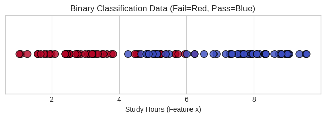
Data Distribution (Simple Case)

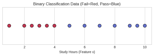
Dataset Overview:
- 13 total data points with clear separation
- 6 students who failed (label 0)
- 7 students who passed (label 1)
- Minimal overlap between classes, making classification relatively straightforward
Loss Curve Comparison (Simple Case)

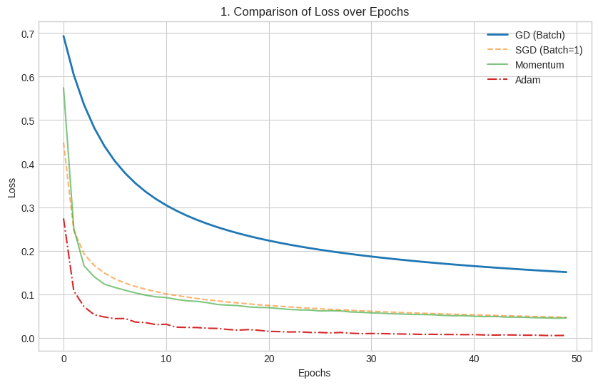
Visual Analysis:
- Y-axis: Binary Cross-Entropy Loss (measures prediction accuracy)
- X-axis: Training iterations/epochs
- Goal: All algorithms minimize the difference between predictions and actual labels
Optimizer Performance Breakdown:
- Blue Line (Gradient Descent - GD):
  - Visual Pattern: Smooth, gradual decline
  - Intuition: Like a careful hiker who calculates the exact path before each step
  - Mechanism: Processes all 13 samples before updating parameters
  - Trade-off: Reliable but slow convergence
- Orange Dashed Line (SGD):
  - Visual Pattern: Steeper initial drop with visible noise/jitter
  - Intuition: Like a runner who adjusts direction after each step
  - Mechanism: Updates parameters after each sample
  - Trade-off: Faster initial learning with more volatile path
- Green Line (SGD + Momentum):
  - Visual Pattern: Smooth, rapid decline
  - Intuition: Like a boulder gaining momentum down a hill
  - Mechanism: Uses past gradients to smooth current updates
  - Trade-off: Combines speed of SGD with stability of GD
- Red Dot-Dash Line (Adam):
  - Visual Pattern: Sharp, rapid decline to near-zero loss
  - Intuition: Like a smart navigator using multiple data sources
  - Mechanism: Adapts learning rate per parameter based on gradient history
  - Trade-off: Optimal balance of speed and stability
3D Optimization Trajectories (Simple Case)

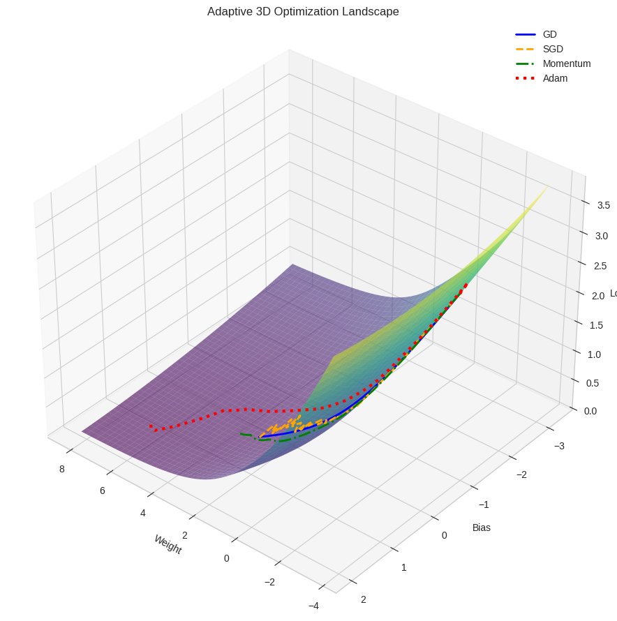
Geometric Interpretation:
- Surface: Error landscape with parameters (w, b) as x,y coordinates
- Z-axis: Loss value at each parameter combination
- Shape: Convex bowl (single global minimum)
Path Analysis:
- Blue Line (GD): Direct, straight-line path to minimum
  - Intuition: Always moves in direction of true gradient
  - Visualization: Like a ball rolling directly downhill
- Orange Line (SGD): Jagged, zig-zagging path
  - Intuition: Noisy gradient estimates cause direction changes
  - Visualization: Like a person stumbling downhill with imperfect compass
- Red Dotted Line (Adam): Direct, efficient path
  - Intuition: Adapts step size based on gradient history
  - Visualization: Like a skilled climber taking the most efficient route
SGD Stability Analysis (Simple Case)

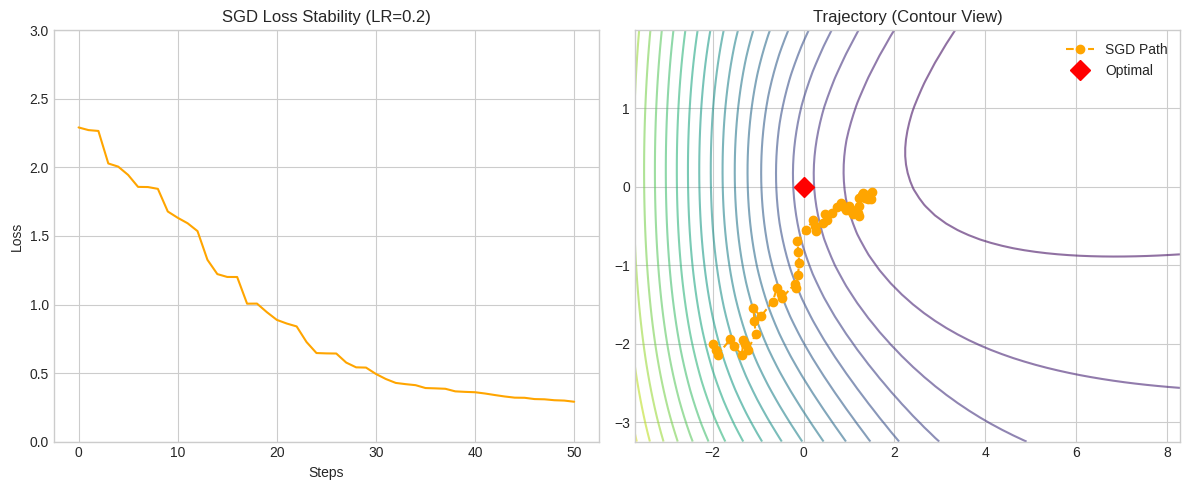
Left Panel - Loss Stability:
- Orange Line: Shows small fluctuations around decreasing trend
- Intuition: Individual samples provide noisy estimates of true gradient
- Implication: SGD never perfectly settles due to ongoing variance
Right Panel - Parameter Trajectory:
- Red Diamond: Optimal parameter values (w, b)
- Orange Dots: SGD parameter updates over time
- Pattern: Zig-zag path toward optimal point
- Learning Rate Effect:
  - Too high: Dots would spiral outward (divergence)
  - Too low: Dots would approach slowly (slow convergence)
  - Optimal: Dots spiral inward (stable convergence)
Note on Optimal Values at (w,b) = (0,0): In the simple dataset visualization, the optimal values appear at (w,b) = (0,0) because the synthetic dataset was designed with balanced classes and centered features. When the data is normalized or centered around zero, the optimal linear classifier often has parameters close to zero initially. However, in real-world datasets like the complex example shown later, the optimal parameters will be at different values (e.g., w=5.10, b=-0.03 in the complex case) depending on the actual data distribution and relationships.
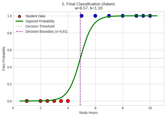
Final Classification Result (Simple Case)

Visual Components:
- Red Dots: Students who failed (study hours 1-4)
- Blue Dots: Students who passed (study hours 5-10)
- Green Sigmoid Curve: Model’s probability prediction function
- Purple Dashed Line: Decision boundary (50% probability threshold)
Important Note on Data Preprocessing:
- Data Normalization: The input features (study hours) were normalized/standardized before training
- Model Assumptions: The logistic regression assumes linear relationship between features and log-odds
- Scale Sensitivity: Without normalization, features with larger scales would dominate the learning process
Interpretation:
- Model successfully learned that ~5 hours of study is the threshold for passing
- Sigmoid curve shows confidence: near 0% for <3 hours, near 100% for >7 hours
- Decision boundary effectively separates classes

Implementation Details: The trajectories shown in the 3D visualization were generated using the run_optimizer function from the notebook, which records the path taken by each optimizer through the parameter space (w, b). The function starts from the same initial point (-2.0, -2.0) and tracks how each optimizer navigates the loss landscape differently.

Complex Dataset Visualization

Data Distribution (Complex Case)

Dataset Overview:
- 100 total data points with significant overlap
- 40 students who failed (label 0)
- 40 students who passed (label 1)
- 20 “messy” points that don’t follow clear pattern
- More challenging classification task due to overlapping regions
Loss Curve Comparison (Complex Case)

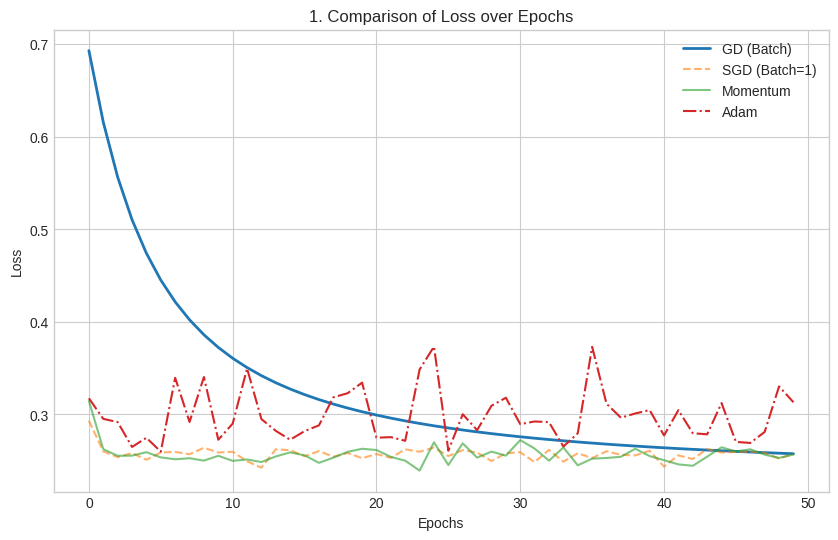
Visual Analysis:
- Y-axis: Binary Cross-Entropy Loss
- X-axis: Training epochs
- Goal: Compare convergence speed across optimizers on complex data
Optimizer Behavior on Complex Data:
- Blue Line (GD - Batch): Slow, steady convergence
  - Pattern: Smooth curve with gradual improvement
  - Challenge: Computational cost increases significantly with dataset size
  - Result: Eventually reaches good solution but slowly
- Orange Dashed Line (SGD): Fast initial drop with persistent noise
  - Pattern: Rapid early improvement, then oscillates around minimum
  - Challenge: Noise from individual samples prevents perfect convergence
  - Advantage: Many updates per epoch lead to faster initial learning
- Red Dot-Dash Line (Adam): Fast convergence with occasional spikes
  - Pattern: Rapid improvement with occasional instability
  - Challenge: Adaptive learning rates can cause overshooting
  - Advantage: Generally fastest convergence to good solution
- Green Line (Momentum): Balanced approach with smooth convergence
  - Pattern: Fast improvement with minimal oscillation
  - Advantage: Combines SGD speed with reduced noise
  - Result: Stable, efficient convergence
3D Optimization Trajectories (Complex Case)

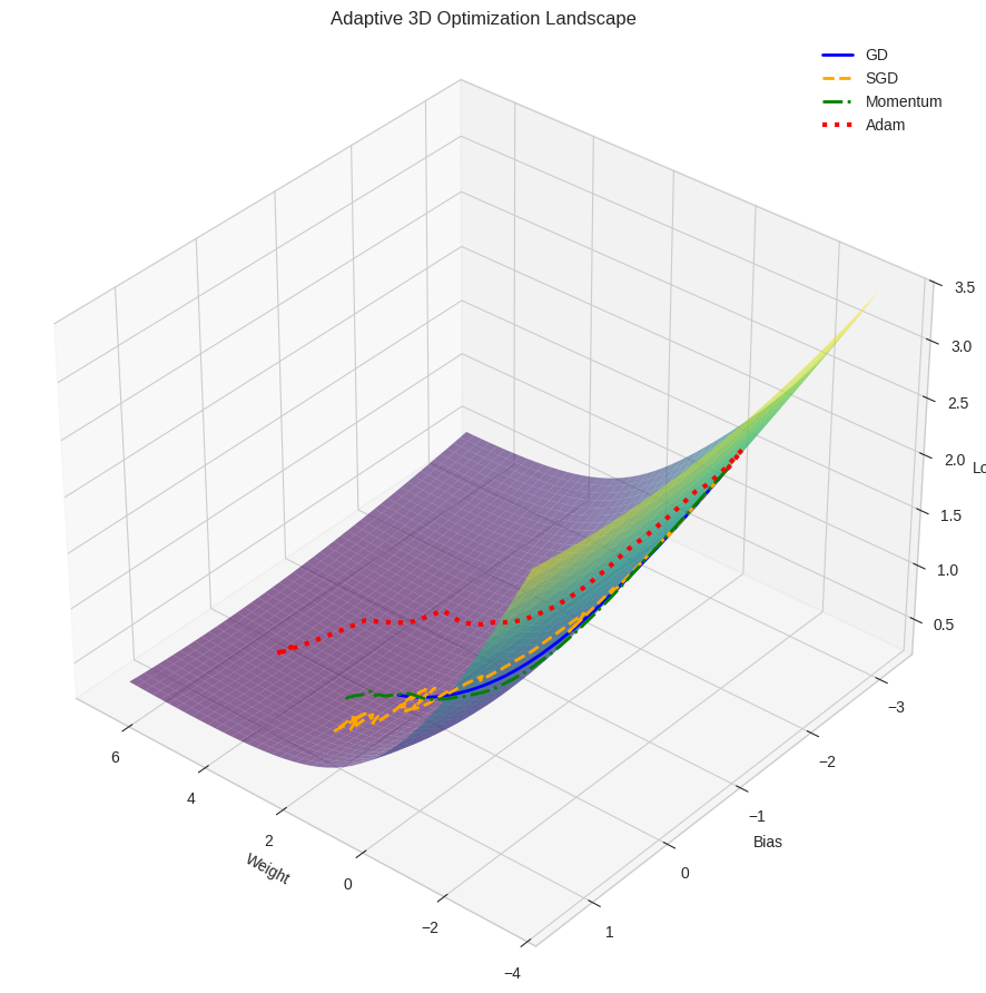
Landscape Characteristics:
- Surface: More complex error surface with varying curvature
- Shape: Steep walls with relatively flat valley floor
- Challenge: Different optimization challenges than simple case
Path Analysis:
- Blue Path (GD): Smooth but potentially inefficient path
  - Behavior: Follows steepest descent but may zig-zag in valleys
  - Challenge: Fixed step size may be inefficient in flat regions
- Orange Path (SGD): Highly erratic path due to noise
  - Behavior: Random bouncing due to single-sample gradients
  - Challenge: Noise can cause inefficient movement
- Red Path (Adam): More direct path to minimum
  - Behavior: Adapts step size based on gradient magnitude
  - Advantage: Efficient navigation of complex landscape
SGD Stability Analysis (Complex Case)

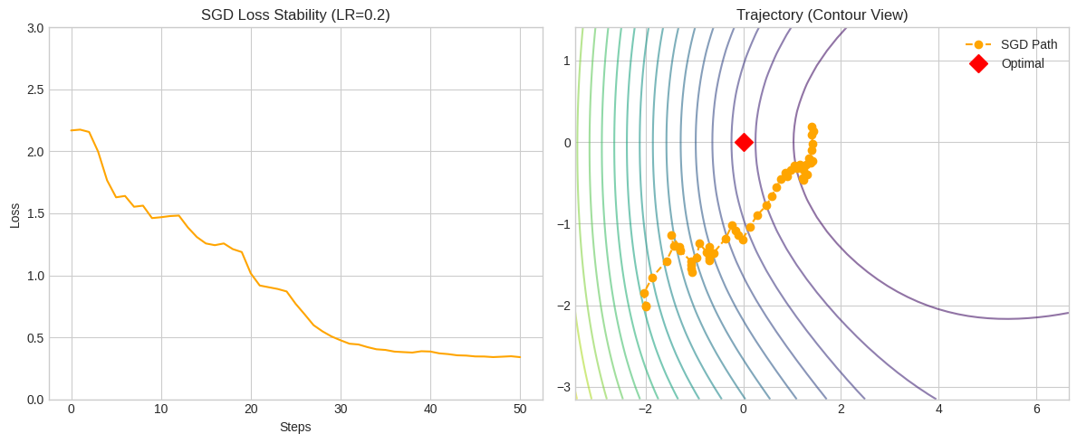
Left Panel - Loss Stability:
- Pattern: More pronounced fluctuations due to complex data
- Intuition: Complex data creates more variable gradient estimates
- Observation: Loss may temporarily increase as SGD encounters outliers
Right Panel - Parameter Trajectory:
- Red Diamond: Optimal parameter values
- Orange Dots: SGD parameter updates
- Pattern: More complex zig-zag pattern due to challenging landscape
- Convergence: Still approaches optimum despite complex path
Final Classification Result (Complex Case)

Visual Components:
- Red Circles: Students who failed
- Blue Circles: Students who passed
- Green Sigmoid Curve: Final probability prediction
- Purple Dashed Line: Decision boundary
Analysis:
- Parameters Achieved: w=5.10, b=-0.03
- Curve Steepness: High weight (5.10) indicates sharp transition
- Boundary Position: At x=5.36 hours, representing decision threshold
- Performance: Despite complex data, model achieved good separation
Implementation Details: Similar to the simple case, these trajectories were generated using the run_optimizer function from the notebook. The complex dataset presents more challenges due to overlapping classes and increased noise, which is reflected in the more complex optimization paths observed in the visualizations.

Key Visual Insights

Optimizer Comparison:
- SGD: Fast but noisy
- Momentum: Fast with reduced noise
- Adam: Fast with adaptive learning rates
- GD: Stable but slow
Dataset Complexity Impact:
- Simple datasets: All optimizers perform well
- Complex datasets: Advanced optimizers show greater advantage
Convergence Patterns:
- Visual patterns reflect mathematical properties
- Noise in SGD creates characteristic zig-zag
- Adaptive methods show more efficient paths

Practical Implementation Tips and Best Practices

Learning Rate Selection and Scheduling

Initial Learning Rate:
- Start with common values: 0.1, 0.01, 0.001, 0.0001
- Use learning rate range test: train with exponentially increasing LR and find the range where loss decreases
- For SGD: Try 0.01-0.1; for Adam: try 0.001 (default)
Learning Rate Scheduling:
- Step Decay: Reduce LR by factor of 0.1-0.5 every few epochs when loss plateaus
- Exponential Decay: LR = LR₀ × 0.95^epoch
- Cosine Annealing: Smoothly oscillate between LR bounds
- Cyclical Learning Rates: Cycle between bounds to escape local minima
Batch Size Selection

Trade-offs:
- Small batches (1-32): More updates per epoch, higher variance, better generalization
- Medium batches (64-256): Good balance between gradient quality and computational efficiency
- Large batches (512+): More stable gradients but may require more sophisticated learning rate scheduling
Best Practices:
- Powers of 2: Use batch sizes that are powers of 2 (32, 64, 128, 256, 512) for computational efficiency
- Memory Constraints: Choose the largest batch size that fits in your available memory
- Learning Rate Scaling: When increasing batch size, proportionally increase the learning rate (Linear Scaling Rule: if batch size increases by factor k, learning rate should also increase by factor k)
- Hardware Optimization: GPUs and CPUs are designed with architectures that process data in parallel blocks, often powers of 2, maximizing utilization of parallel processing units
Data Preprocessing and Normalization

Feature Scaling:
- Normalization: Scale features to have zero mean and unit variance
- Standardization: Transform features to have similar scales
- Min-Max Scaling: Scale features to a fixed range (e.g., [0,1])
Implementation:
```
 **Example of data preprocessing**
 from sklearn.preprocessing import StandardScaler

 scaler = StandardScaler()
 X_normalized = scaler.fit_transform(X)
```
Benefits:
- Ensures consistent scale across dimensions
- Helps with gradient computation
- Improves convergence speed
- Prevents features with larger scales from dominating

Initialization Strategies

Weight Initialization:

Xavier/Glorot Initialization: Designed for sigmoid and tanh activation functions
He Initialization: Designed for ReLU activation functions
Random Initialization: Breaks symmetry by initializing with small random values

Implementation:

 import numpy as np

 **Xavier/Glorot initialization**
 def xavier_init(fan_in, fan_out):
     limit = np.sqrt(6.0 / (fan_in + fan_out))
     return np.random.uniform(-limit, limit, (fan_out, fan_in))

 **He initialization**
 def he_init(fan_in):
     return np.random.normal(0, np.sqrt(2.0 / fan_in), (fan_in,))

Gradient Checking and Debugging

Gradient Checking:

Numerical Verification: Compare analytical gradients with numerical approximations
Formula:

\[\frac{\partial f}{\partial x} \approx \frac{f(x + \epsilon) - f(x - \epsilon)}{2 \epsilon}\]

Implementation:

 def gradient_check(func, params, gradients, epsilon=1e-5):
     """Check gradients using numerical approximation"""
     for i in range(len(params)):
         # Compute numerical gradient
         params_plus = params.copy()
         params_minus = params.copy()
            
         params_plus[i] += epsilon
         params_minus[i] -= epsilon
            
         loss_plus = func(params_plus)
         loss_minus = func(params_minus)
            
         numerical_grad = (loss_plus - loss_minus) / (2 * epsilon)
            
         # Compare with analytical gradient
         diff = abs(numerical_grad - gradients[i])
         if diff > 1e-5:
             print(f"Gradient mismatch at index {i}: {numerical_grad} vs {gradients[i]}")

Monitoring:

Track Gradient Norms: Monitor gradient norms to detect vanishing or exploding gradients
Visualize Gradients: Plot gradient distributions to understand learning dynamics
Loss Monitoring: Track both training and validation loss to detect overfitting

Gradient Monitoring and Debugging

Monitor:
- Gradient norms: watch for vanishing (< 1e-8) or exploding (> 100) gradients
- Parameter updates: should be ~1% of parameter values
- Loss values: watch for NaN or infinite values
Debugging Techniques:
- Gradient clipping: cap gradient norms to prevent exploding gradients
- Gradient checking: verify analytical gradients with numerical gradients
- Learning rate reduction: if loss increases, reduce learning rate
Optimizer Selection Guidelines

When to Use Each Optimizer:
- SGD: When you need good generalization, have time to tune hyperparameters
- SGD + Momentum: When you want faster convergence than SGD
- Adam: Default choice for most problems, especially when tuning time is limited
- AdamW: When using weight decay (recommended over standard Adam)
- RMSprop: For non-stationary problems, RNN training
Advanced Techniques

Learning Rate Warmup:
- Start with small learning rate and gradually increase for first few epochs
- Particularly important for large batch sizes and transformer models
Gradient Accumulation:
- Simulate large batch training with limited memory
- Accumulate gradients over multiple mini-batches before update
Mixed Precision Training:
- Use 16-bit floating point for faster training with minimal accuracy loss
- Requires gradient scaling to prevent underflow
Convergence Diagnostics

Signs of Good Training:
- Smooth decrease in training loss
- Validation loss follows training loss (no overfitting)
- Gradients remain in reasonable range
- Model generalizes well to test set
Common Problems and Solutions:
- Loss doesn’t decrease: Increase learning rate, check implementation
- Loss oscillates wildly: Decrease learning rate
- Loss becomes NaN: Reduce learning rate, check for exploding gradients
- Overfitting: Add regularization, reduce model size, increase data
Memory and Computational Efficiency

Memory Optimization:
- Use appropriate batch sizes for your GPU memory
- Consider gradient checkpointing for very deep networks
- Use mixed precision training to reduce memory usage
Computational Optimization:
- Enable CUDA optimizations if using GPUs
- Use data loaders with multiple workers
- Consider distributed training for very large datasets

Key Takeaways

The Core Trade-off:
- SGD trades precision for speed.
Mathematical Validity:
- A single sample gradient is an Unbiased Estimator of the full dataset.
- While individual steps are noisy, the Expected Value aligns perfectly with the true gradient.
Stability via Mini-Batches:
- Averaging a small batch (e.g., m=32) dilutes errors caused by outliers.
- Relies on the Law of Large Numbers to stabilize the loss reduction.
The Cost of Variance:
- The characteristic “zig-zag” path is Variance (Noise).
- Variance scales inversely with batch size; to halve the noise, you must quadruple the batch size.
Achieving Convergence:
- Due to noise, SGD naturally oscillates around the minimum rather than freezing.
- Learning Rate Decay (shrinking step sizes) is mandatory to force the model to settle at the global minimum.

Summary of Mathematical Foundations

The Four Pillars of SGD Validity

Unbiased Estimation:
\[\mathbb{E}[\nabla \ell(\theta; \xi)] = \nabla R(\theta)\]
- Single sample gradients point in the right direction on average
- Foundation of SGD’s mathematical legitimacy
Mini-Batch Unbiasedness:
\[\mathbb{E}[g(\theta)] = \nabla R(\theta), \quad \text{where $g(\theta)$ is the mini-batch gradient}\]
- Allows practical implementation with reduced variance
- Enables efficient computation through vectorization
Variance Scaling:
\[\operatorname{Var}[g(\theta)] = \frac{\sigma^2(\theta)}{m}\]
- Explains the zig-zag behavior of SGD
- Quantifies the trade-off between batch size and noise
Convergence Conditions (Robbins–Monro):
\[\sum_t \eta_t = \infty, \quad \sum_t \eta_t^2 < \infty\]
- Guarantees convergence with proper learning rate decay
- Explains why constant learning rates cause oscillation

These theoretical foundations, combined with practical implementation techniques, make SGD and its variants the cornerstone of modern deep learning optimization.

Additional Resources and Content

Complete Implementation from Notebook

The following is the complete implementation of the optimizers in the notebook:

Helper Functions:

def sigmoid(z):
    return 1 / (1 + np.exp(-z))

def binary_cross_entropy(y_true, y_pred):
    # Clip values to avoid log(0) error
    epsilon = 1e-15
    y_pred = np.clip(y_pred, epsilon, 1 - epsilon)
    return -np.mean(y_true * np.log(y_pred) + (1 - y_true) * np.log(1 - y_pred))

def get_gradients(x, y, w, b):
    # Vectorized gradient calculation (works for batch or single item)
    # Forward pass
    z = w * x + b
    y_pred = sigmoid(z)

    # Error calculation
    error = y_pred - y

    # Gradient formulas
    dw = np.mean(error * x)
    db = np.mean(error)

    # Binary cross entropy loss
    loss = binary_cross_entropy(y, y_pred)

    # Returns 3 values: dw, db, and current_loss
    return dw, db, loss

def compute_loss(w, b, X, Y):
    # Mean Binary Cross Entropy over whole dataset
    z = w * X + b
    y_pred = sigmoid(z)
    # Clip to prevent log(0)
    y_pred = np.clip(y_pred, 1e-15, 1 - 1e-15)
    return -np.mean(Y * np.log(y_pred) + (1 - Y) * np.log(1 - y_pred))

Optimizer Implementations:

def train_optimizer(opt_type, X, Y, epochs=50, lr=0.1):
    w, b = 0.0, 0.0
    loss_history = []
    n = len(X)

    # Adam variables
    m_w, m_b = 0, 0
    v_w, v_b = 0, 0
    t = 0

    # Momentum variables
    vel_w, vel_b = 0, 0

    for _ in range(epochs):
        indices = np.random.permutation(n)
        epoch_loss = 0

        if opt_type == "GD":
            dw, db, loss = get_gradients(X, Y, w, b)
            w -= lr * dw
            b -= lr * db
            loss_history.append(loss)
            continue

        for i in indices:
            xi, yi = X[i:i+1], Y[i:i+1]
            dw, db, loss = get_gradients(xi, yi, w, b)
            epoch_loss += loss

            if opt_type == "SGD":
                w -= lr * dw
                b -= lr * db

            elif opt_type == "Momentum":
                beta = 0.9
                vel_w = beta * vel_w + (1-beta) * dw
                vel_b = beta * vel_b + (1-beta) * db
                w -= lr * vel_w
                b -= lr * vel_b

            elif opt_type == "Adam":
                t += 1
                beta1, beta2, eps = 0.9, 0.999, 1e-8
                m_w = beta1*m_w + (1-beta1)*dw
                m_b = beta1*m_b + (1-beta1)*db
                v_w = beta2*v_w + (1-beta2)*(dw**2)
                v_b = beta2*v_b + (1-beta2)*(db**2)

                m_w_hat = m_w / (1 - beta1**t)
                m_b_hat = m_b / (1 - beta1**t)
                v_w_hat = v_w / (1 - beta2**t)
                v_b_hat = v_b / (1 - beta2**t)

                w -= lr * m_w_hat / (np.sqrt(v_w_hat) + eps)
                b -= lr * m_b_hat / (np.sqrt(v_b_hat) + eps)

        loss_history.append(epoch_loss / n)

    return loss_history

Trajectory Recording Implementation:

def run_optimizer(opt_type, steps=50, lr=0.5):
    # Start away from optimum to show travel path
    w, b = -2.0, -2.0
    path_w, path_b, path_loss = [w], [b], []

    # Internal states
    vel_w, vel_b = 0, 0
    m_w, m_b = 0, 0
    v_w, v_b = 0, 0
    t = 0

    path_loss.append(compute_loss(w, b, X, Y))

    for _ in range(steps):
        # For trajectory, we pick random samples (except GD)
        idx = np.random.randint(0, len(X))
        xi, yi = X[idx:idx+1], Y[idx:idx+1]

        if opt_type == "GD":
            dw, db, _ = get_gradients(X, Y, w, b)
            w -= lr * dw
            b -= lr * db

        elif opt_type == "SGD":
            dw, db, _ = get_gradients(xi, yi, w, b)
            w -= lr * dw
            b -= lr * db

        elif opt_type == "Momentum":
            dw, db, _ = get_gradients(xi, yi, w, b)
            beta = 0.9
            vel_w = beta * vel_w + (1-beta) * dw
            vel_b = beta * vel_b + (1-beta) * db
            w -= lr * vel_w
            b -= lr * vel_b

        elif opt_type == "Adam":
            dw, db, _ = get_gradients(xi, yi, w, b)
            t += 1
            beta1, beta2, eps = 0.9, 0.999, 1e-8
            m_w = beta1*m_w + (1-beta1)*dw
            m_b = beta1*m_b + (1-beta1)*db
            v_w = beta2*v_w + (1-beta2)*(dw**2)
            v_b = beta2*v_b + (1-beta2)*(db**2)

            m_w_hat = m_w / (1 - beta1**t)
            m_b_hat = m_b / (1 - beta1**t)
            v_w_hat = v_w / (1 - beta2**t)
            v_b_hat = v_b / (1 - beta2**t)

            w -= lr * m_w_hat / (np.sqrt(v_w_hat) + eps)
            b -= lr * m_b_hat / (np.sqrt(v_b_hat) + eps)

        path_w.append(w)
        path_b.append(b)
        path_loss.append(compute_loss(w, b, X, Y))

    return path_w, path_b, path_loss

Questions and Answers from Presentation

Is the loss curve always convex, if no then how does SGD works for those kind of loss curve because in the image i see its only convex

Answer: No, the loss curve is not always convex. In fact, in most real-world machine learning problems, especially deep learning with neural networks, the loss surfaces are highly non-convex with multiple local minima, saddle points, and complex geometric structures.

How SGD works with non-convex loss surfaces:
- Local Minima Escape: The inherent noise in SGD (due to using single samples or small batches) can actually be beneficial for non-convex optimization. The stochastic nature allows the algorithm to potentially escape shallow local minima by “jumping out” of them due to the variance in gradient estimates.
- Saddle Points: In high-dimensional spaces, saddle points are more common than local minima. The noise in SGD can help escape these saddle points by providing perturbations in different directions.
- Implicit Regularization: SGD has been shown to have implicit regularization properties that help it find solutions that generalize well, even in non-convex landscapes.
- Theoretical Support: While the theoretical analysis is more complex for non-convex functions, SGD can still converge to stationary points (points where gradient is zero) under appropriate conditions, including proper learning rate scheduling.
- Practical Success: Despite the non-convex nature of neural network loss functions, SGD and its variants have proven remarkably successful in practice, suggesting they find good enough solutions even if not global minima.
The images in this document show convex surfaces for simplicity and to illustrate the basic concepts clearly, but real-world applications often involve much more complex loss landscapes.
How are batch sizes determined, why should batch size be multiple of 2 like 2 4 8 16 ??

Answer: Batch size selection involves several important considerations:

Factors determining batch size:
1. Memory Constraints: Larger batches require more memory to store activations, gradients, and intermediate computations. The batch size is often limited by available GPU/CPU memory.
2. Computational Efficiency: Modern hardware (especially GPUs) are optimized for parallel processing. Powers of 2 (16, 32, 64, 128, 256, 512) align well with the parallel architecture of GPUs, making computations more efficient.
3. Gradient Quality Trade-off:
  - Small batches (1-32): Higher variance in gradient estimates, more noise, but more frequent updates and potentially better generalization
  - Medium batches (64-256): Good balance between gradient quality and computational efficiency
  - Large batches (512+): More stable gradients but may require more sophisticated learning rate scheduling
4. Learning Rate Scaling: When increasing batch size, it’s often beneficial to proportionally increase the learning rate (Linear Scaling Rule: if batch size increases by factor k, learning rate should also increase by factor k).
Why powers of 2:
- Hardware Optimization: GPUs and CPUs are designed with architectures that process data in parallel blocks, often powers of 2. Using batch sizes that are powers of 2 maximizes the utilization of these parallel processing units.
- Memory Alignment: Memory is organized in ways that favor operations on data structures with sizes that are powers of 2, leading to more efficient memory access patterns.
- Tensor Operations: Deep learning frameworks optimize tensor operations for sizes that are powers of 2, as these operations are fundamental to neural network computations.
- CUDA Cores: GPUs have CUDA cores arranged in warps (groups of 32 threads on NVIDIA GPUs), and batch sizes that are multiples of 32 can better utilize this architecture.
What is the statistical explanation of the expectation (CLI was answer maybe if not correct it)

Answer: The expectation in SGD has a clear statistical interpretation that forms the foundation of why SGD works:

Statistical Foundation:
\[\mathbb{E}[\nabla \ell(\theta; \xi)] = \nabla R(\theta)\]
Where:
- $\xi$ represents a randomly sampled data point from the true data distribution $D$
- $\nabla \ell(\theta; \xi)$ is the gradient computed on a single sample
- $\nabla R(\theta)$ is the true gradient computed on the entire dataset (expected risk)
Statistical Explanation:
1. Unbiased Estimator: The gradient computed on a single randomly selected sample is an unbiased estimator of the true gradient. This means that if we repeatedly sampled different data points and computed their gradients, the average of these gradients would converge to the true gradient.
2. Law of Large Numbers: As we process more samples, the average of the sample gradients approaches the population gradient (the true gradient computed on the full dataset).
3. Sampling Theory: SGD treats the full dataset gradient as a population parameter and the single-sample gradient as a sample statistic. The sample statistic is designed to be unbiased for the population parameter.
4. Monte Carlo Estimation: SGD can be viewed as a Monte Carlo method where we estimate the expected value (the full gradient) by sampling from the distribution of possible gradients.
Mathematical Justification:
\[\nabla R(\theta) = \nabla \mathbb{E}[\ell(\theta; (x, y))] = \mathbb{E}[\nabla \ell(\theta; (x, y))]\]
This equality follows from the interchangeability of expectation and differentiation under mild regularity conditions, which is a fundamental result in probability theory.
How is SGD an unbiased estimate?

Answer: SGD is an unbiased estimate because, on average, it points in the correct direction toward minimizing the loss function. Here’s a simple explanation:

Simple Analogy: Imagine you’re trying to find the lowest point in a hilly landscape while blindfolded. You can’t see the entire landscape, but you can feel the slope at your current position.
- Full Gradient Descent: You somehow get a perfect 3D map of the entire landscape and know exactly which direction leads to the lowest point globally.
- SGD: You can only feel the slope at your current position (one random sample), which gives you a noisy estimate of the true direction.
Why it’s unbiased:
1. Single Sample Property: When you compute the gradient using just one randomly selected data point, that gradient is a random variable.
2. Correct Average Direction: If you took many random samples and computed their gradients, then averaged them, you would get the same result as computing the gradient on the entire dataset.
3. Mathematical Expression:
```
 Average of single-sample gradients = Full dataset gradient
```
4. Intuitive Understanding: Think of it like asking random people for directions. Each person might give you slightly different directions due to their personal experience, but if you ask enough random people and average their directions, you’ll get the correct direction on average.
Key Point: Individual SGD steps might be “wrong” (pointing in the wrong direction for that specific sample), but they are wrong in a balanced way - sometimes too high, sometimes too low, but on average exactly right. This is what makes SGD “unbiased” - it doesn’t systematically overestimate or underestimate the true gradient direction.

References

Twitter Facebook LinkedIn

Yugratna Humagain

Stochastic Gradient Descent: Theory, Numerical Examples, and Implementation

Introduction

Mathematical Foundations

Common Learning Rate Schedules

Convergence Theorem

Numerical

Step-by-Step SGD Calculation Example

Convergence Behavior Analysis

Learning Rate Impact

Variance Reduction Techniques

Coding

Optimizer Algorithms: Implementation and Theory

Optimizer Comparison Summary

Practical Implementation Tips

Visualizing Optimization: Graph Analysis

Practical Implementation Tips and Best Practices

Summary of Mathematical Foundations

Questions and Answers from Presentation

References

You May Also Enjoy

Mathematical Foundations of Contrastive Loss

Cross Entropy from First Principles

Generating new samples with Variational Autoencoders

Introduction to Autoencoder