Satellite Image Analysis
Interpretation and analysis of remote sensing imagery involves the identification and/or measurement of varied targets in an image so as to extract useful information from them. During image analysis, we need to be careful regarding false topographic perception like flowing of river from lower regions to higher etc. Similarly the satellite image does not provide true color image unless the hyperspectral image is used. Here we will be studying about digital processing and analysis only. It basically involves:
- Preprocessing
- Image Enhancement
- Image Transformation
- Image Classification and Analysis
1. Preprocessing
Georeferencing
Converting the captured image to geo referenced data is called georeferencing, and also known as geometric correction, image registration. In order to georeference images, we need to take a reference point known as Ground Control Points (GCP). GCP are fixed points in the map which are visible in both real world and the image to be referenced. The GCP can be identified using the landmark points, google earth or any referenced map which has been georeferenced previously. The accuracy of GCP is relevant to spatial resolution. Usually bridge, mountain peaks are considered as GCP. Transformation is done using least square fit using different order of polynomials. The order of polynomials determines the number of GCP to be used. Mathematically,
Minimum $GCP = (p+1)(p+2)/2$
Where $p$ is the order of the polynomial. Usually for more accuracy we take twice the value of minimum GCP.
The error between the original pixel and transformed pixel can be calculated using euclidean distance. If the root mean square (RMS) is less than the spatial resolution, then it means the introduced error is less than 1px. This is considered to be almost errorless. For e.g. for a 50m spatial resolution image, if the RMS is 49, then it is almost effortless.
Once the image is georeferenced, the distortions are removed. The distortion might be due to earth rotation, altitude variation, spacecraft velocity, yaw variation etc.
Sampling
After georeferencing, the image and new image grid are overlaid. In order to calculate the pixel value on the new image grid we use algorithms like nearest neighbour, bilinear interpolation, cubic interpolation, spline interpolation etc. Usually bilinear interpolation is used for the interpolation since it requires less computation than cubic and spline interpolation and does not create artifacts like from nearest neighbour.
Atmospheric correction is done to remove the effect of atmosphere in the image like clouds, haze over a region with reference to ground data. This is usually done for small regions since larger areas have different climate conditions and the same atmospheric correction might not be feasible.
2. Image Enhancement techniques
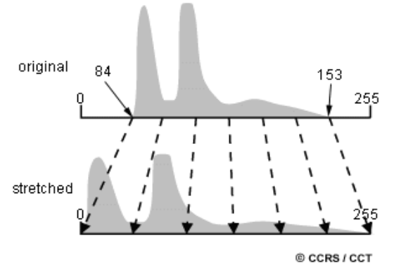
In order to make visual interpretation and understanding of imagery easier, we perform different enhancements on an image. In raw imagery, the useful data often populates only a little portion of the available range of digital values (commonly 8 bits or 256 levels). We basically stretch the image histogram to use more available range and thus help locate targets. A histogram may be a graphical representation of the brightness values that comprise a picture . So if we plot it in a graph with brightness values in X-axis and frequency in Y-axis, we get a graph as shown in figure.
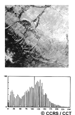
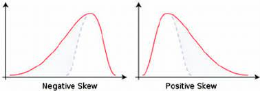
Histogram can be positively or negatively skewed based on the frequency of pixel value. The negatively skewed histogram represents the higher number of higher pixel values while positively skewed represents the lower pixel values. The histogram can be used for thresholding operations.
Similarly we might have multiple peaks in the histogram in real world images. The multiple peaks in satellite images represents the multiple types of source available in the ground. For e.g. if a satellite image consists of water body and vegetation, then it will have multiple peaks in the histogram. So, if we select the proper band they can be separable using histogram only. Along with this, histogram of multispectral bands can be used since each region has different reflectivity in different bands resulting in different histograms of the same bodies.
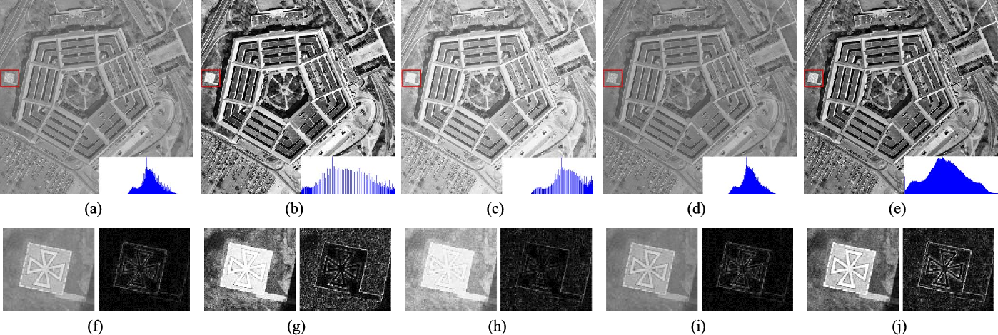
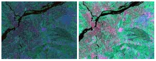
One of the simplest types of enhancement is a linear contrast stretch. Here we find the minimum and the maximum brightness values and then apply a transformation to stretch this range to fill the full range. This enhances the contrast in the image with light toned areas appearing lighter and dark areas appearing darker, making visual interpretation much easier.
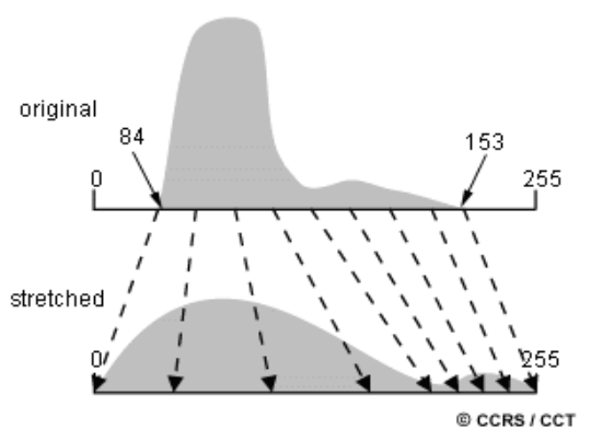
If the image is not uniformly distributed or if we need to enhance a certain target only we can use histogram-equalized stretch. Here we assign more display values to the frequently occurring portion of histogram.
For example, suppose we’ve a picture of the mouth of a river, and let the water portions of the image occupy the digital values from 40 to 76 out of the whole image histogram. If we wished to reinforce the detail within the water, perhaps to work out variations in sediment load, we could stretch only that tiny portion of the histogram represented by the water (40 to 76) to the total grey level range (0 to 255). All pixels below or above these values would be assigned to 0 and 255, respectively, and therefore the detail in these areas would be lost. However, the detail within the water would be greatly enhanced.
Spatial Filtering
Spatial filters are designed to highlight or suppress specific features in an image based on their spatial frequency. Spatial frequency refers to the frequency of the variations in tone that appear in an image. “Rough” textured areas of an image, where the changes in tone are abrupt over a small area, have high spatial frequencies, while “smooth” areas with little variation in tone over several pixels, have low spatial frequencies.
A low-pass (smoothing) filter emphasizes larger, homogeneous areas of similar tone and reduces the smaller detail in an image. Thus, low-pass filters generally smoothen the appearance of an image. Low pass filter basically includes:
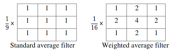
a. Averaging linear filters: gives the average of the pixels contained in the neighborhood of the filter mask. For example: standard average and weighted average filter.
b. Order-statistics nonlinear filters: nonlinear spatial filters whose response is based on ordering (ranking) the pixels contained in the neighborhood. Examples include Max, Min, and Median filters.
Example: Consider the following $5x5$ image:
| 20 | 25 | 55 | 81 | 100 |
| 31 | 27 | 81 | 111 | 110 |
| 250 | 251 | 77 | 70 | 120 |
| 30 | 30 | 80 | 100 | 130 |
| 40 | 50 | 90 | 125 | 140 |
Apply a $3x3$ median filter, we get
| 20 | 25 | 55 | 81 | 100 |
| 31 | 27 | 81 | 111 | 110 |
| 250 | 251 |
77 | 70 | 120 |
| 30 | 30 | 80 | 100 | 130 |
| 40 | 50 | 90 | 125 | 140 |
Sorted: 27, 30, 30, 31, 77, 80, 81, 250, 251
So our result is:
| 20 | 25 | 55 | 81 | 100 |
| 31 | 27 | 81 | 111 | 110 |
| 250 | 77 |
77 | 70 | 120 |
| 30 | 30 | 80 | 100 | 130 |
| 40 | 50 | 90 | 125 | 140 |
High-pass filters do the opposite and serve to sharpen the appearance of fine detail in an image. Directional, or edge detection filters are designed to highlight linear features, such as roads or field boundaries.
These filters can also be designed to enhance features which are oriented in specific directions. These filters are useful in applications such as geology, for the detection of linear geologic structures.
3. Image Transformation
Image transformation involves manipulation of multiple bands of data to produce a new image that highlights features that are not in the original image. We can calculate the correlation matrix among the bands and use uncorrelated bands for analysis. Along with that we can take the ratio of two bands, also known as band ratio, of image and also create false color composite based on it which can produce new information to reveal.
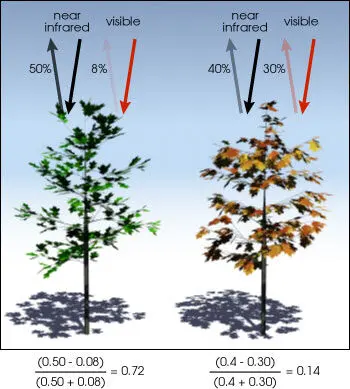
- NDVI One of the mostly used techniques is the Normalized Difference Vegetation Index(NDVI). NDVI quantifies the vegetation by measuring the difference between near-infrared and red light.
$NDVI = \frac{NIR - Red}{NIR + RED}$
Healthy vegetation (containing more chlorophyll) reflects more near-infrared (NIR) and green light compared to other wavelengths. But it absorbs more red and blue lights. This leads to higher NDVI for healthy vegetation and lower for unhealthy vegetation. The NDVI index is between [-1, 1]. This can be used to analyze the vegetation of an area over a time.
4. Image Classification
Image classification can be done in the satelite image to classify different parts/theme (like: water, coniferous forest, decidious forest, corn, wheat, etc.). The result image will have mosaic of pixels, each o fwhich belong to which theme.
Common classification procedures can be broken down into two broad subdivisions based on the method used: supervised classification and unsupervised classification. In supervised classification, we basically have labelled data of terrain and develop a model based on it so it predicts accurately input satellite images. For example if we have a training examples with water bodies labelled, our model will predict the water bodies in new images.
In unsupervised learning, we have unlabeled data, so our model will itself find clusters of similar pixels. So here any pixel that looks similar are grouped in same class irrespective of what they actually represent.
Co-Authors: Shital Adhikari and Anil Kumar Shrestha