Vector Spaces and Subspaces

This is a one of several posts in Linear Algebra series. All the posts are available here. I assume you are familiar with vectors if not please refer Introduction to Vectors.

In this post we will start by introducing vector spaces and subspaces, then explore pivot columns, free columns and rank that we will need in the next post. Finally, we will find a complete solution of $Ax = b$.

Before we dive into Vector spaces let’s see what field is.

Field: Formally, a field is an algebraic structure with set of elements and two operations (called multiplication and addition) which follows the following strict properties called field axioms, which in itself is a separate topic in itself, which hopefully will be covered later in this linear algebra series.

Intuitively, let $a, b$ $\varepsilon$ $\mathbb{R}$, then $a + b, a - b, a.b$ and $\frac{a}{b}$ all belongs to $\mathbb{R}$ (given that $b \not ={0}$). So, we say $\mathbb{R}$ is a Field. Similarly, $\mathbb{Q}$ and $\mathbb{C}$ are also fields. But are $\mathbb{N}$, $\mathbb{Z}$ fields? For example, $2$ and $5$ are in $\mathbb{N}$ but $2 - 5$ is not. So clearly, they are not a field.

Now we are good to discuss vector spaces. A nonempty set V of elements $\vec{a}, \vec{b}, \vec{c}…$ is called a vector space if there are two defined algebraic operations:

I. Vector addition $(\vec{a} + \vec{b})$ should satisfy following axioms:

1. Commutative: $\vec{a} + \vec{b} = \vec{b} + \vec{a}$
2. Associative: $(\vec{a} + \vec{b}) + \vec{c} = \vec{a} + (\vec{b} + \vec{c)}$
3. There is a unique vector, zero vector ($\vec{0}$), in V such that, $\vec{a} + \vec{0} = \vec{a}$
4. For every $\vec{a}$ in V there is a unique vector in V that is denoted by $-\vec{a}$ such that, $\vec{a} + -\vec{a} = \vec{0}$

II. Scalar multiplication If c and k are any scalar, then c$\vec{a}$ should satisfy:

1. Distributive: $c(\vec{a} + \vec{b}) = c\vec{a} + c\vec{b}$
2. Distributive: (c + k)$\vec{a}$ = c$\vec{a}$ + k$\vec{a}$
3. Associative: c(k$\vec{a}$) = (ck)$\vec{a}$
4. For every $\vec{a}$ in V, 1$\vec{a}$ = $\vec{a}$

Let’s start with something that everyone is familiar with: $\mathbb{R}^2$, which is a XY-plane. In fact this is a vector space containing all column vectors $\vec{v}$ with 2 components. For $3$ components, we have $\mathbb{R}^3$ vector space that we live in. That said, we can generalize it to:

$\mathbb{R}^n$ to be a vector space of all column vectors with n components.

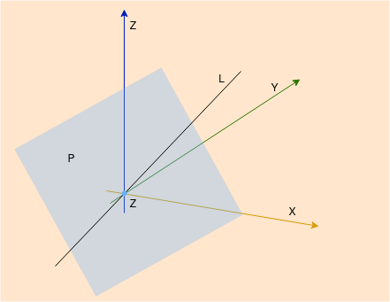
Now if we consider just a plane through origin in the vector space $\mathbb{R}^3$ such that adding two vectors in the plane results to a vector in the same plane and multiplying by any scalar also results in a vector in the same plane. Hence the plane is a vector space in $\mathbb{R}^3$, we call it Subspace. The plane has 3 components so it can not be considered as $\mathbb{R}^2$. Similarly, a line through origin in $\mathbb{R}^3$, a point at origin (zero vector) and $\mathbb{R}^3$ are also a subspace. The plane $P$ and line $L$ is shown in the figure below.

$P$ and $L$ are subspaces, but what about their union and intersections. Do they form a subspace?

• $P \cup L$ is not a subspace.
• $P \cap L$ is actually a zero vector so it’s a subspace.

If plane $P1$ and plane $P2$ are subspaces in $\mathbb{R}^3$ as shown in the figure.

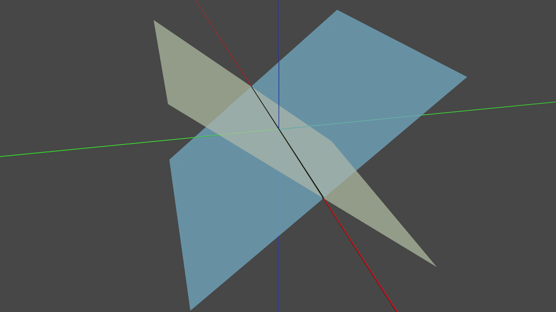
• $P1 \cup P2$ is not a subspace.
• $P1 \cap P2$ is actually one dimensional line and any linear combination of vectors inside the line will give vector within the line so it’s a subspace.

Row Space, Column Space and Null Space

The row space, $R(A)$ is a set of vectors that contains all the linear combinations of rows of a matrix and the column space, $C(A)$ is a set of vectors that contains all the linear combinations of columns. The row space and column space are subspaces in $\mathbb{R}^n$ and $\mathbb{R}^m$ respectively for a matrix with $m$ rows and $n$ columns. Then if we have,

\[Ax = \begin{bmatrix} 1 & 2 \\ 3 & 4\\ 5 & 6 \end{bmatrix} \begin{bmatrix} x_1\\ x_2\end{bmatrix}\]

1. Row space of A is a subspace of $\mathbb{R}^2$.
2. Column space of A is a subspace of $\mathbb{R}^3$. The column space of all combinations of the two columns fills up a plane in $\mathbb{R}^3$ as it has only 2 columns.

In the equation $Ax = b$, if we take all their linear combinations, this gives the column space of $A$. So if b is in that column space, we can solve the equation $Ax = b$.

What if $b = 0$ ? The immediate solution we get is $x = 0$. This is the only solution for invertible matrices but for non-invertible matrices, there are nonzero solutions along with zero and belongs to a space. We call this space a Null space, N(A). As the solution vector $x$ has $n$ components, the nullspace is a subspace of $\mathbb{R}^n$. The solutions obtained are called special solutions when $Ax = 0$.

But when $b \not ={0}$, does the solution $x$ form a subspace? No, because $x = 0$ does not solve the equation and hence the solution does not have zero vector.

More on fundamental subspaces is discussed here

Pivot Columns and Free Columns

To understand these, let’s suppose a system of linear equation,

\[x_1 + 2x_2 + 2x_3 + 2x_4 = b_1\] \[2x_1 + 4x_2 + 6x_3 + 8x_4 = b_2\] \[3x_1 + 6x_2 + 8x_3 + 10x_4 = b_1\]

So we get the matrix $A$ and perform elimination to get echelon form,

\[A = \begin{bmatrix} 1& 2& 2 & 2 \\ 2& 4& 6& 8 \\ 3 & 6 & 8 & 10\end{bmatrix}\] \[R_2 = 2*R_1 - R_1, R_3 = 3*R_1 - R_2\] \[U = \begin{bmatrix} 1& 2 & 2 & 2 \\ 0 & 0 & 2 & 4 \\ 0& 0& 2& 4 \end{bmatrix}\] \[R_3 = R_3 - R_2\] \[U = \begin{bmatrix} 1& 2 & 2 & 2 \\ 0 & 0 & 2 & 4 \\ 0& 0& 0& 0 \end{bmatrix}\]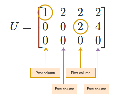

Here $C_1$ and $C_3$ are pivot columns and $C_2$ and $C_4$ are free columns. So we see that the number of pivot columns is $2$ and the number of free columns is (number of columns - number of pivot columns)$ = 2$. This generalizes to the fact that if $Ax = 0$ has more unknowns than equations $(n > m)$, then there must be at least one free column.

Rank of a matrix

Rank ($r$) of a matrix is the number of pivots. Rank of a matrix gives almost all information about the solutions. This shows that there are $r$ independent rows and columns in the given matrix. This also deals with spaces of vectors: the rank of a matrix is $r$ means, the column and row space are in $r$ dimensions. And the dimension of null space is $n-r$.

The rank for above mentioned matrix $A$ = the number of pivots = $2$. So it’s column space and row space is in $2$-dimension and null space is in $4-2 = 2$ dimension.

Now for a $m$ x $n$ matrix $A$ of rank $r$, let’s see what happens when $r = m$, $r = n$, $r = m = n$, and $r < m$, $r < n$.

1. Full column rank, $(r = n)$: Here every column has pivot. So there is no free variable and hence the Null space $N(A)$ will have only the zero vector. This results in $X = X_{particular}$ if it exists.

   \[A = \begin{bmatrix}1 & 3\\ 2 & 1 \\ 6 & 1 \\ 5 & 1\end{bmatrix}\] \[R = \begin{bmatrix}1 & 0 \\ 0 & 1 \\ 0 & 0 \\ 0&0\end{bmatrix}\] \[R = \begin{bmatrix}I \\ 0\end{bmatrix}\]

2. Full row rank, $(r = m)$: Here every row has pivots and $n - r$ or $n - m$ free variables. So here we can solve $Ax = b$ for every $b$.

   \[A = \begin{bmatrix}1 & 2& 6 & 5 \\ 3 & 1 & 1 & 1\end{bmatrix}\] \[R = \begin{bmatrix}1 & 0 & F \\ 0 & 1\end{bmatrix}\] \[R = \begin{bmatrix}I & F\end{bmatrix}\]

3. Full rank $(r =m = n)$: Here since $r = m = n$, the matrix is a square and is invertible. So,

   \[R = I\]

   And the Null space $N(A)$ has only zero vector.

In a nutshell, we get the following table.

Full rank (r = m = n)	Full column rank(r = n < m)	Full row rank (r = m < n)	r < m < n
$R = I$	\(R = \begin{bmatrix}I \\ 0\end{bmatrix}\)	$R = \begin{bmatrix}I & F\end{bmatrix}$	\(R = \begin{bmatrix}I & F \\ 0 & 0\end{bmatrix}\)
1 solution	0 or 1 solution	$\infty$ solutions	$0$ or $\infty$ solutions

Solving Ax = b

The goal of this section is to find the complete solution of $Ax = b$ if it has a solution. Let’s use the linear system from earlier.

\[x_1 + 2x_2 + 2x_3 + 2x_4 = b_1\] \[2x_1 + 4x_2 + 6x_3 + 8x_4 = b_2\] \[3x_1 + 6x_2 + 8x_3 + 10x_4 = b_1\]

Checking the solvability

The solvability condition is: If combinations of rows of $A$ gives zero row, then the same combinations of the entries of b must give zero. In fact this corresponds to what we already know, $Ax = b$ is solvable when b is in the Column space C(A).

From the above equations we can obtain our augmented matrix and perform elimination:

\[\begin{bmatrix} 1& 2& 2 & 2 & b_1 \\ 2& 4& 6& 8 & b_2\\ 3 & 6 & 8 & 10 & b_3\end{bmatrix}\] \[\begin{bmatrix} 1& 2& 2 & 2 & b_1 \\ 0& 0& 2& 4& b_2 - 2b_1\\ 0 & 0 & 2 & 4 & b_3 - 3b_1\end{bmatrix}\] \[\begin{bmatrix} 1& 2& 2 & 2 & b_1 \\ 0& 0& 2& 4& b_2 - 2b_1\\ 0 & 0 & 0 & 0 & b_3 - b_2 - b_1\end{bmatrix}\]

As we see in $R_3$, the combinations of rows is zero row (that is 0 = 0, so the equation can be solved.), then we must have

$b_3 - b_2 - b_1 = 0$.

Then for $b_1 = 1, b_2 = 8, b_3 = 9$, we get $b_3 - b_2 - b_1 = 0$.

So now we know that the solution exists. In order to find the complete solution we will,

1. Find $X_{particular}$:

   • Set all free variables to zero.
   • Solve $Ax = b$ for pivot variables.
2. Find $X_{null space}$
3. $X_{complete}$ = $X_{particular}$ + $X_{null space}$

Finding $X_{particular}$

This is quite straightforward, we set free vaiables as $0$ i.e. $X_2 = 0$ and $X_4 = 0$, so the system becomes,

\[x_1 + 2x_3 = 1\] \[2x_3 = 8\]

And after back substitution, we get $x_3 = 4$ and $x_1 = -7$. Our one particular solution is

\[X_{particular} = \begin{bmatrix}-7\\0\\4\\0\end{bmatrix}\]

Finding $X_{nullspace}$

To find our solution in null space let’s start with our matrix $A$ and perform elimination to get reduced row echelon form.

\[A = \begin{bmatrix} 1& 2& 2 & 2 \\ 2& 4& 6& 8 \\ 3 & 6 & 8 & 10\end{bmatrix}\] \[U = \begin{bmatrix} 1& 2 & 2 & 2 \\ 0 & 0 & 2 & 4 \\ 0& 0& 0& 0 \end{bmatrix}\]

Here $C_1$ and $C_3$ are pivot columns and $C_2$ and $C_4$ are free columns. So if we set free variables $x_2 = 1$ and $x_4 =0$, we get

\[x_1 + 2 + 2x_3 = 0\] \[2x_3 = 0\]

which gives $x_1 = -2, x_3 = 0$.

Similarly, if we set $x_2 = 0$ and $x_4 =1$, we get $x_1 = 2$ and $x_3 = -2$

We finally get the whole Null space,

\[X_{null} = c_1\begin{bmatrix}-2\\1 \\ 0 \\ 0\end{bmatrix} + c_2\begin{bmatrix}2\\ 0 \\ -2 \\ 1\end{bmatrix}\]

for any constant $c_1$ and $c_2$.

Now if we take $U$ to reduced row-echelon form $R$,

\[R_2 = R_2/2\] \[R = \begin{bmatrix}1& 2 & 2 & 2\\ 0 & 0 & 1 & 2 \\ 0 & 0& 0& 0\end{bmatrix}\] \[R_1 = R_1-2*R_2\] \[R = \begin{bmatrix}1 & 2 & 0& -2\\ 0 & 0 & 1 & 2 \\ 0 & 0& 0& 0\end{bmatrix}\]

This reduced row echelon form has a structure: Identity matrix in pivot columns, free matrix in free column and zeros below.

\(R = \begin{bmatrix}I & F\\ 0 & 0\end{bmatrix}\) with \(I = \begin{bmatrix}1 & 0 \\ 0 & 1\end{bmatrix}\), \(F = \begin{bmatrix}2 & -2 \\ 0 & 2\end{bmatrix}\)

We can notice here that the Null space is actually in the form:

\[X_{null} = c\begin{bmatrix}-F \\ I\end{bmatrix}\]

Complete Solution $X_{complete}$

Now we have both $X_{particular}$ and $X_{nullspace}$ and hence our complete solution is:

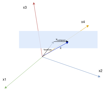
\[X_{complete} = \begin{bmatrix}-7\\0\\4\\0\end{bmatrix} + c_1\begin{bmatrix}-2\\1 \\ 0 \\ 0\end{bmatrix} + c_2\begin{bmatrix}2\\ 0 \\ -2 \\ 1\end{bmatrix}\]

Plotting the solution we get,

For further reading please refer here.

References

1. Introduction to Linear Algebra, W. G. Strang
2. What is Vector space ? (Toronto)
3. Notes on Discrete Mathematics (Yale)
4. The Four Fundamental Subspaces (IITM)
5. TheFourFundamentalSubspaces (MIT)