

Eigen Values and Eigen Vectors
Eigenvalues and Eigen Vectors
Almost all vectors change direction when they are multiplied by a transformation matrix suppose $A$. There are certain vectors $x$ that will give same direction when multiplied by $A$ and will be stretched by some scalar $\lambda$. Thus, the vector $x$ is called the eigen vector and the scalar $\lambda$ is called the eigen value.
They can be represented mathematically as:

Here, Matrix $A$ acts by stretching the vector $x$, not changing its direction, so $x$ is an eigenvector of $A$.
To solve $Ax=\lambda x$, we can rewrite the equation as $(A-\lambda I)x=0$. This will have a non zero solution if matrix $(A-\lambda I)$ is singular. For singular matrix we know that it’s determinant is zero. Therefore,
\[|A-\lambda I|=0\]- Now, we solve for $\lambda$ first.
- Next, for each eigen value $\lambda$ we solve $|A-\lambda I|=0$ to find the eigen vector $x$.
For example,
-
We have a matrix \(A=\begin{pmatrix} -6 & 3 \\ 4 & 5 \end{pmatrix}\)
-
Then, $|A-\lambda I|=0$,
\[\Bigg|\begin{pmatrix} -6 & 3 \\ 4 & 5 \end{pmatrix}-\lambda \begin{pmatrix} 1 & 0 \\ 0 & 1 \end{pmatrix}\Bigg|=0\] - Calculating the determinants we get, $(-6-\lambda)(5-\lambda)-3 \times 4=0$, quadratic equation $\lambda^{2}+\lambda -42=0$, and solving it we get $\lambda=-7$ or $6$
- For eigen value $\lambda=6$, use the equation $Ax=\lambda x$ to find its corresponding eigen vector and for eigen value $\lambda=-7$ we use the same equation to find its corresponding eigen vector.
For $\lambda$ = $6$,
\[\begin{pmatrix} -6 & 3 \\ 4 & 5 \end{pmatrix}\begin{pmatrix} x \\ y \end{pmatrix}=6\begin{pmatrix} x \\ y \end{pmatrix}\]. After multiplying we get these two equations: $-12x+3y=0$ and $4x-y=0$. Either equation reveals that $y = 4x$, so the eigenvector is any non-zero multiple of this:
\(\begin{pmatrix} 1 \\ 4 \end{pmatrix}\).
Similarly, for $\lambda=-7$ the eigen vector is :
\[\begin{pmatrix} -3 \\ 1 \end{pmatrix}\]Some useful properties:
- For $n\times n$ matrix the product of $n$ $\lambda$s equals the determinant of that matrix.
- The sum of $n$ $\lambda$s = sum of $n$ diagonal entries.
-
Sum of diagonal entries of a matrix is called the trace of that matrix.
$\lambda_1 + \lambda_2 +…\lambda_n$= trace =$a_{11}+a_{22}+…a_{nn}$ - The eigen values might not be real numbers even if the matrix is real. For example a 90 degree rotation matrix
\(Q=\begin{pmatrix} 0 & -1 \\ 1 & 0 \end{pmatrix}\)
has no real eigen values. It’s eigen values are $\lambda_1=i$ and $\lambda_2=-i$
- The eigen values of a triangular matrix will always lie along its diagonal. For example
\(A=\begin{pmatrix}
3 & 1 \\ 0 & 3
\end{pmatrix}\)
It’s eigen values are
$\lambda_1=3$ and $\lambda_2=3$. Since, it has repeated eigen value it will have only one independent eigen vector which is
\(\begin{pmatrix} 1 \\ 0 \end{pmatrix}\)
Diagonalization of a matrix
Suppose we gave $n$ independent eigen vectors of matrix $A$ and let’s put them in columns,
$AX=$
\[A \begin{pmatrix} \vert & \vert & & \vert \\ X_{1} & X_{2} & \ldots & X_{n} \\ \vert & \vert & & \vert \end{pmatrix}\] \[= \begin{pmatrix} \vert & \vert & & \vert \\ \lambda_1X_{1} & \lambda_2X_{2} & \ldots & \lambda_nX_{n} \\ \vert & \vert & & \vert \end{pmatrix}\]\(= \begin{pmatrix}
\vert & \vert & & \vert \\
X_{1} & X_{2} & \ldots & X_{n} \\
\vert & \vert & & \vert
\end{pmatrix}\)
\(\begin{pmatrix}
\lambda_{1} & & \\
& \ddots & \\
& & \lambda_n
\end{pmatrix}\)
\(=X\Lambda\)
Here, $\Lambda$ is the diagonal eigen value matrix. To make $X$ invertible it must be independent. So,
\[AX=X\Lambda\] \[A=X\Lambda X^{-1}\]This diagonalization is a factorization technique of a matrix.
Rules for diagonalization:
- For a matrix, if the eigenvectors for $n$ different eigen values are independent then only we can diagonalize that matrix.
- If the eigen values are repeated then there might be few independent eigen vectors for the corresponding eigen values, in such case a matrix cannot be diagonalized. For example:
Since, it is triangular matrix, it’s eigen values are the diagonal ones $\lambda_1,\lambda_2=5$. This will have only one independent eigen vector i.e.
\[\begin{pmatrix} 1 \\ 0 \end{pmatrix}\]Thus matrix $A$ cannot be diagonalized.
The $k^{th}$ power of a matrix $A$ is $A^{k}=X\Lambda^{k}X^{-1}$. If matrix $A$ is squared or raised to any power $k$ then the eigen values also gets squared or get raised to the power $k$ but eigen vectors remains the same.
Symmetric Matrices
A symmetric matrix is a square matrix that is equal to its transpose, $A=A^{T}$. Because equal matrices have equal dimensions, only square matrices can be symmetric. So, we now want to explore what is special about $AX = \lambda$ when $A$ is symmetric?
If a matrix is symmetric then it will have:
- Real eigen values
- Perpendicular eigenvectors (orthogonal eigenvectors) that we can choose to convert to unit vector to produce orthonormal eigenvectors.
- Why do we use the word “choose”? Because the eigenvectors do not have to be unit vectors. Their lengths are at our disposal. We will choose unit vectors-eigenvectors of length one, which are orthonormal and not just orthogonal.
Previously a matrix $A$ if diagonalizable could be written as $A=X\Lambda X^{-1}$, where $X$ is independent eigenvector matrix, $\Lambda$ is the diagonal eigen value matrix and $X^{-1}$ is the inverse of the eigen vector matrix.
Now, if $A$ becomes symmetric then it can be factorized as $A=Q\Lambda Q^{-1}$ = $Q\Lambda Q^{T}$ , where $\Lambda$ is real eigenvalue matrix , $Q$ is orthonormal eigenvector matrix and we know that for orthonormal matrix $Q^{T}=Q^{-1}$. This makes us easier to factorize $A$ because we do not need to find the inverse of $Q$ but instead find $Q^{T}$ which is much more computationally easier to find.
Eigen values and pivots:
If a matrix is symmetric then the products of pivots = determinant = product of the eigenvalues. This will give the relation that the number of positive eigenvalues of a symmetric matrix equals the number of positive pivots.
For example, a symmetric matrix
after row reduction
\[A=\begin{pmatrix} 1 & 3 \\ 0 & -8 \end{pmatrix}\]This matrix has pivots 1 and -8 and eigenvalues 4 and -2.
Therefore,
- Number of positive eigen values= number of positive pivots.
- Product of eigenvalues=$4\times(-2)=-8$, product of pivots= $1\times(-8)=-8$, Determinant=$1-(3\times3)=-8$.
In non symmetric matrix repeated $\lambda$s produce shortage of eigen vectors. But, in symmetric matrix there is no repeated $\lambda$s so no shortage of eigenvectors. Therefore, symmetric matrix is always diagonalizable.
System of differential equations
The main aim of this section is to convert constant coefficient differential equation into linear algebra.
A simple first order differential equation $\frac{du}{dt}=\lambda u$ are solved by the exponentials. Therefore, its solution will be $u(t)=Ce^{\lambda t}$.
For the initial condition, let ordinary equation $\frac{du}{dt}= u$, then $u(t)=Ce^t$. At initial condition $t=0$ so, $e^0=1$. Thus, $u(0)=C$.
Therefore the solution can be rewritten as: $u(t)=u(0)e^\lambda t$. This is the case for 1 by 1 problem.
Linear algebra moves to $n\times n$. So, system of n equations become $\frac{du}{dt}=Au$ with initial condition vector given as: $u(0)=\begin{pmatrix}
u_1(0)
.
.
u_n(0)
\end{pmatrix}$.
Here, A is a constant $n\times n$
matrix and $u$ is a vector whose components are the unknown functions in the system.
The linear constant coefficient equations are solved by exponentials $e^{\lambda t}$, when $Ax=\lambda x$. Where, $\lambda$ is the eigen value of $A$ and $x$ is the eigen vector.
Therefore, the general solution for $\frac{du}{dt}=Au(t)$ for a $n\times n$ system is given as :
For example:
We need to convert the differential equation
\[2y''+5y'-3y=0\]with the initial conditions:$y(0)=-4, y’(0)=4$ into a system and solve the system and use this solution to get the solution to the original differential equation.
-
We first write the 2nd order differential equation as a system of first order, linear differential equations.
$x_1=y, x_1’=y’=x_2$
$x_2=y’$
$x_2’=y’’=\frac{3}{2}y-\frac{5}{2}y’=\frac{3}{2}x_1-\frac{5}{2}x_2$
-
The system then becomes:
-
The eigen values of the matrix let \(A=\begin{pmatrix} 0 & 1 \\ \frac{3}{2} & \frac{-5}{2} \end{pmatrix}\) is $\lambda_1=-3, \lambda_2=0.5$ and thier corresponding eigen vectors are \(\begin{pmatrix} 1 \\ -3 \end{pmatrix}\) and \(\begin{pmatrix} 2 \\ 1 \end{pmatrix}\)
-
The general solution is then, \(x(t)=c_1e^{-3t}\begin{pmatrix} 1 \\ -3 \end{pmatrix} + c_2e^{0.5t}\) \(\begin{pmatrix} 2 \\ 1 \end{pmatrix}\)
-
Using the initial condition the value of constants $c_1, c_2$ is determined:
$c_1=\frac{-22}{7}, c_2=\frac{-3}{7}$
- The actual solution to the system is then, \(x(t)=\frac{-22}{7}e^{-3t}\begin{pmatrix} 1 \\ -3 \end{pmatrix}-\frac{-3}{7}e^{0.5t} \begin{pmatrix} 2 \\ 1 \end{pmatrix}\)
-
\[x(t)=\begin{pmatrix}
y(t) \\
y^{'}(t)
\end{pmatrix}\]
the solution to the original differential equation is just the top row of the solution to the matrix system. The solution to the original differential equation is then,
\(y(t)=\frac{-22}{7}e^{-3t}\begin{pmatrix} 1 \\ -3 \end{pmatrix}-\frac{-3}{7}e^{0.5t} \begin{pmatrix} 2 \\ 1 \end{pmatrix}\).In this case, the bottom row should be the derivative of the top row.
The 3 important properties of a solution:
(Note: When $\lambda$ is complex, then its real part will always determine if the solution grows or decays)
- The solution will grow or blow up if all the real eigen values $\lambda s>0$, when $t\rightarrow \infty$
- The solution will be in a steady state or always in the same direction if one the eigen values i.e $\lambda_1=0$ and the rest of the real part of eigen values is negative i.e $\lambda s<0$, when $t\rightarrow \infty$.
- The solution will be stable/decays when real $\lambda s <0$ as $t\rightarrow \infty$.
We can also write the solution $u(t)$ in new form i.e $u(t)=e^{At}u(0)$. If $A$ has $n$ independent eigen vectors then it can be diagonalized. Therefore, $e^{At}$ can be written as $Xe^{\Lambda t}X^{-1}$.Thus, the solution $u(t)$ is now written as:
\[u(t)=Xe^{\Lambda t}X^{-1}u(0)\]Positive Definite Matrices
Given a symmetric two by two matrix \(\begin{pmatrix} a & b \\ b & c \end{pmatrix}\)
here are four ways to tell if it’s positive definite:
- Eigenvalue test: $\lambda_1> 0$,$\lambda_2> 0$. If the eigen values are positive.
- Determinants test: $a > 0$, $ac − b^{2} > 0$. If all the sub determinants are positive.
- Pivot test: $a > 0$, $\frac{ac-b^{2}}{a}> 0$. If all the pivots are positive.
- $x^{T}Ax>0$ for every non zero vector $x$.
$x^{T}Ax$= \(\begin{pmatrix} x & y \end{pmatrix} \begin{pmatrix} a & b \\ b & c \end{pmatrix}\begin{pmatrix} x \\ y \end{pmatrix}=ax^{2}+2bxy+by^{2}>0\)
For Positive semidefinite matrices, they must have eigenvalues greater than or equal to 0.
Some examples and test for minimum:
The matrix \(\begin{pmatrix} 2 & 6 \\ 6 & 20 \end{pmatrix}\)
is positive definite – its determinant is 4 and its trace is 22 so its eigenvalues are positive. It’s quadratic form associated with it is given by:
\[x^{T}Ax=\begin{pmatrix} x & y \end{pmatrix} \begin{pmatrix} 2 & 6 \\ 6 & 20 \end{pmatrix}\begin{pmatrix} x \\ y \end{pmatrix}=2x^{2}+12xy+20y^{2}>0\]The graph of this function is shown below:
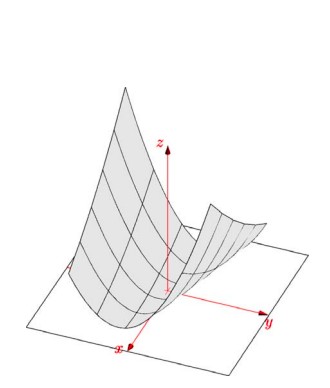
The graph of the above function $2x^{2}+12xy+20y^{2}$ is like a bowel shape and has minima only at origin.
The matrix \(\begin{pmatrix} 2 & 6 \\ 6 & 7 \end{pmatrix}\) is a non positive definite. It’s quadratic form associated with it is given by:
\[x^{T}Ax=\begin{pmatrix} x & y \end{pmatrix} \begin{pmatrix} 2 & 6 \\ 6 & 7 \end{pmatrix}\begin{pmatrix} x \\ y \end{pmatrix}=2x^{2}+12xy+7y^{2}<0\]The graph of this function is shown below:
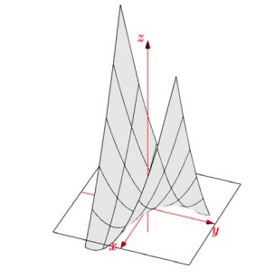
The graph shows that the function $2x^{2}+12xy+20y^{2}$ has saddle point.
From the above two examples we’ve learned that if a matrix is positive definite then its function will have a minima and if it is not positive definite then its function will have a saddle point instead of minima. Finding the minima of any function is often important, specially in optimization problems.
We know that for a function having minima its first derivative is 0. But, this also applies for non positive definite matrix. Therefore, it is the second derivative that is required and it must be positive; the slope must be increasing.
The matrix of second derivatives of $f (x, y)$ is:
\[\begin{pmatrix} f_{xx} & f_{xy} \\ f_{yx} & f_{yy} \end{pmatrix}\]and is called Hessian matrix.This matrix is symmetric because $f_{xy} = f_{yx}$. Its determinant is positive when
the matrix is positive definite, which matches the $f_{xx} f_{yy} > f^{2}_{xy}$ test for a minimum that we learned in calculus.
Thus,a function of several variables $f (x_1, x_2, …, x_n)$ has a minimum when its matrix
of second derivatives is positive definite.