BERT (Bidirectional Encoder Representation From Transformers)

Introduction

2018 was a breakthrough year in NLP, Transfer learning, particularly models like Allen AI’s ELMO, OPENAI’s transformer, and Google BERT was introduced [1]. Due to this, NLP Community got pretrained models which was able to produce SOTA result in many task with minimal fine-tuning. Due to the development of such pre-trained models, it’s been referred to as NLP’s ImageNet moment, referencing how years ago similar developments accelerated the development of machine learning in Computer vision tasks. This is a momentous development since it enables anyone building a machine learning model involving language processing to use this powerhouse as readily available component saving the time, energy, knowledge, and resources that would have gone to training a language-processing model from scratch [4].
BERT (Bidirectional Encoder Representation From Transformer) is a transformers model pretrained on a large corpus of English data in a self-supervised fashion. This means it was pre-trained on the raw texts only, with no humans labelling which is why it can use lots of publicly available data.

BERT works in two steps:

1. Pre-training:
   • In pretraining phase, it uses large amount of unlabeled data to learn a language representation in an unsupervised fashion.
   • Hence in pre-training phase, we will train a model using a combination of Masked Language Modelling (MSM) and Next Sentence Prediction (NSP) on a large corpus.
2. Fine-tuning:
   • In Fine-tuning phase, we will use a learned weights from pre-trained models in a supervised fashion using a small amount of labeled datasets.

Example: Spam Classification

• The most straight-forward way to use pretrained BERT is to use it to classify a single piece of text as shown: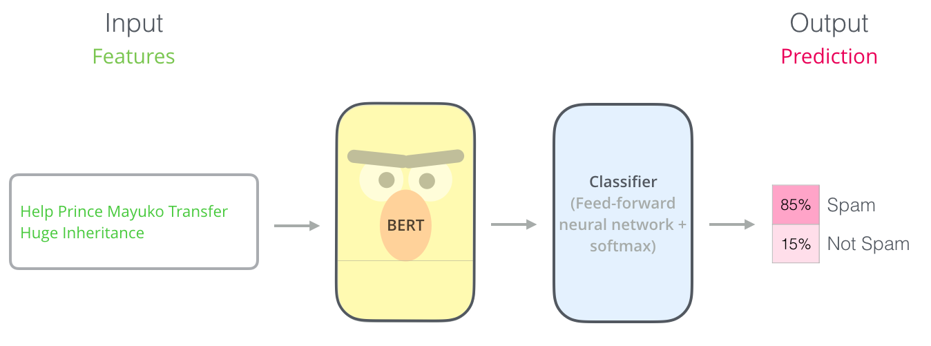
  • 

    Image taken from the illustrated BERT

  • In above scenario, we used pretrained BERT model and we added feedforward neural network followed by softmax activation on top of pretrained model for spam classification task.
  • This way of modifying pre-trained architecture based on our requirements is known as fine-tuning.

Before diving into the details of BERT, let’s get familiar with transfer learning which will be helpful in understanding BERT.

Transfer Learning

When training a certain models, the common desirable goals are:

• Reduce training time
• Faster Convergence
• Improve predictions
• Small Datasets

We can achieve the above-defined goals, not 100% but near to it with a technique called transfer learning. So a question may arise what really transfer learning is? and the answer is, It is a machine learning technique where a model trained on one task is repurposed on a second related task. The main approach of transfer learning is select source task, develop source model, reuse model, and tune model. If you want to learn more about transfer I recommend you to visit A Gentle introduction to Transfer Learning

Now we know a high overview of transfer learning. In the coming section, we will try to understand how transfer learning helps to leverage the power of highly available unlabeled textual data.

Labeled Vs Unlabeled Data

There are lots of unlabeled data available compared to the labeled text data. So, for pre-training we can use unlabeled data and train the pretrain model. Now we use a pre-trained model which has a learned weight to a new task with labeled data. This is a very useful way to make use of highly available unlabeled text data to a supervised learning task where we work with labeled text data.

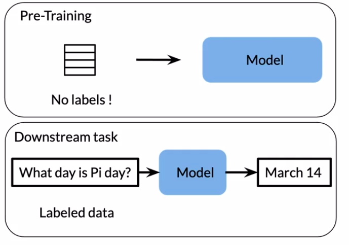
Image taken from NLP specialization

As I have said earlier that, we will train a model using unlabeled data, so one question may be popping around your head i.e What is the task that we will use an unlabeled data to train our model? and the answer is Mask language modeling (MLM) and Next sentence prediction (NSP). So, inorder to understand MLM and NSP just keep on reading.

Now, let’s look at the BERT architecture mentioned in the BERT paper. Under the hood, mentioned architectures are based on how many transformer encoders are used. If you are new to transformer then its time to redirect you to the cool transformer blog i.e. the illustrated transformer

Model Architecture

BERT model provided in the paper came in two sizes i.e. BERT BASE and BERT LARGE.

• BERT BASE: Comparable in size to the OPENAI’s transformer inorder to compare performance.
• BERT LARGE: A ridiculously huge model which achieved the state of the art results reported in the paper.

Comparison Table

• 

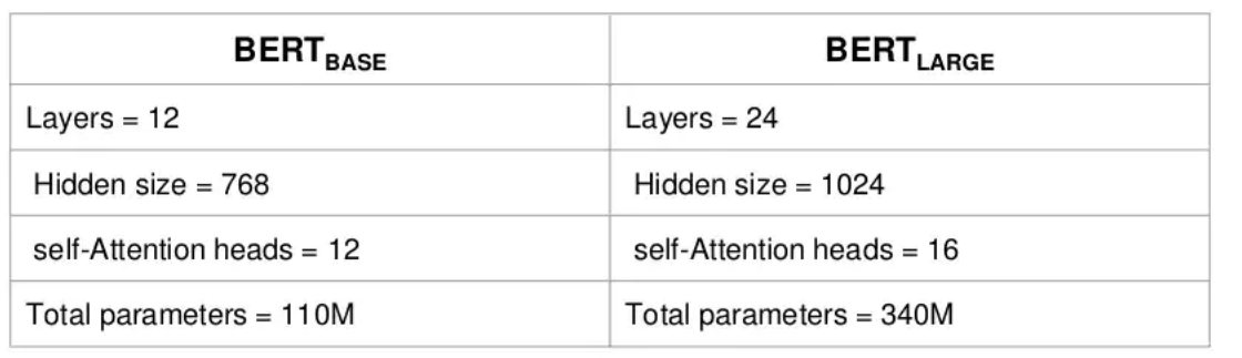
  Image taken from slide share

• Layers: Number of transformer encoder i.e. 12 for the Base version, and 24 for the Large version.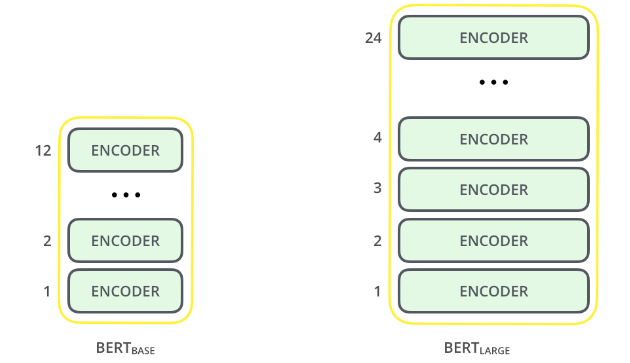
• 

  Image taken from the illustrated BERT

• Hidden size: Number of neurons in fully-connected layer of transformer encoder i.e. 768 hidden units for the Base version and 1024 hidden units for the Large version.
• Self-Attention heads: Number of self-attention in each transformer encoder i.e. 12 self-attention heads for the Base version and 16 self-attention heads for the Large version.

BERT: Input/Output Representation

As we have discussed, BERT is a pre-trained model, so it expects input data in a specific format. In the below section, we will understand how to formalize raw input sentences before feeding them to the BERT model.

Special Tokens

• BERT can take as input either one or two sentences, and uses the two special token i.e.
  • [SEP] token to differentiate two input sentences.
  • [CLS] token always appears at the start of the text, and is useful to sentence level classification tasks (Spam Classification).
• Both tokens are always required even if we only have one sentence, and even if we’re not using BERT for classification.

• Example:

  [CLS] BERT makes use of wordpiece tokenization. [SEP] We will see it in below section.
  
  [CLS] BERT makes use of wordpiece tokenization. [SEP]
  

Tokenization

Tokenization is a way of separating a piece of text into smaller units called tokens. Here, tokens can be either words, characters, or subwords.

BERT makes use of WordPiece tokenization i.e. the BERT tokenizer was created with a WordPiece model. This model greedily creates a fixed-size vocabulary (python dictionary) of individual characters, subwords, and words that best fits our language data. The generated vocabulary contains:

1. Whole words
2. Subwords occuring at the front of a word or in isolation ("em" as in "embeddings" and the standalone sequence of characters "em" as in "go get em")
3. Subwords not at the front of a word, which are preceded by '##' to denote this case
4. Individual characters

To tokenize a word under this model, the tokenizer first check if the whole word is in the vocabulary. If not, it tries to break the word into the largest possible subwords contained in the vocabulary, and as a last resort will decompose the word into individual characters. As a result, rather than assigning out of vocabulary words to catch all token like 'OOV' or 'UNK', words that are not in the vocabulary are decomposed into subword and character tokens.

• Example: embeddings is represented as ["em", "##bed", "##ding", "##s"]

Formalizing Input

Each input token to the BERT is the sum of Token embeddings, Segment embeddings, and Position embeddings.

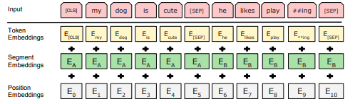
Image taken from BERT paper

• Position Embeddings
  • Similar to the transformer, we will feed all the word sequences in the input sentence at once to the BERT model. So to identify the position of words in an input sentence i.e. where each word is located in the input sentence, we will generate position embeddings.
• Segment Embeddings
  • BERT is trained on and expects sentence pairs, so segment embeddings help to indicate whether a sentence is first or second.
  • Segment Embeddings is important because we also accomplish the Next Sentence Prediction task in BERT pretraining phase.
  • So, if you want to process two sentences, assign each word in the first sentence plus the [SEP] token a series of 0’s, and all tokens of the second sentence a series of 1’s.
• Token Embeddings
  • It is basically an initial low-level embedding of tokens.
  • Initial low-level embedding is essential because the machine learning model doesn’t understand textual data.

Finally, we are ready for BERT. In the below section, we will look into 3 different ways how the BERT model can be used i.e. Pre-training, Fine-Tuning, and Feature extraction.

BERT: Pretraining

During the pretraining phase, the BERT model is trained on unlabelled textual data over different tasks like Masked Language Modeling and Next Sentence Prediction.

Masked Language Modeling (MLM)

In masked language modeling, the model randomly chooses 15% of the words in the input sentence and among those randomly chosen words, mask them 80% of the time (i.e. using [MASK] token from vocabulary), replace them with a random token 10% of the time, or keep as is 10% of the time and the model has to predict the masked words in the output. This is different from traditional recurrent neural networks (RNNs) that usually see the words one after the other i.e. sequentially, or autoregressive models like GPT which internally mask the future tokens. It allows the model to learn a bidirectional representation of the sentence. So, in MLM we are actually inputting an incomplete sentence and asking BERT to complete it for us which is analogous to fill in the blanks.

Image taken from the illustrated BERT

Next Sentence Prediction (NSP)

In the Next Sentence Prediction task, Given two input sentences, the model is then trained to recognize if the second sentence follows the first one or not. This helps the BERT model handle relationships between multiple sentences which is crucial for a downstream task like Q/A and Natural language inference. So, for NSP while constructing training data, 50% of the inputs are actual pairs with label [IsNext], and 50% of the inputs have random sentences with label [NotNext].

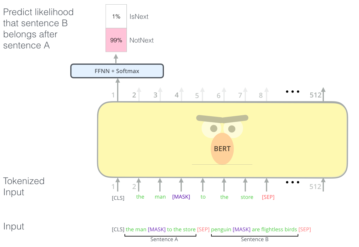
Image taken from the illustrated BERT

Hence, During the Pre-training phase, the BERT model is trained for two tasks i.e. MLM and NSP simultaneously on large textual data i.e. the BookCorpus(800M words), and English wiki (2,500M words). The model parameters are then optimized by backpropagating combined loss i.e. Cross-Entropy for masked language modeling and Binary Cross Entropy for next sentence prediction. In this way, the model learns an inner representation of the English language that can then be used as either Fine-Tuning or Feature extractor which we will discuss in the coming section.

BERT: Fine-tuning

The main idea of fine-tuning is to use learned weight from the pre-training phase in downstream tasks with minimal task-specific architecture adjustment so that training will be inexpensive relative to the pre-training phase. In the BERT literature, we can see that using this concept BERT is able to achieve state of the art result in eleven downstream tasks namely Question and Answering, Natural Language Inference, and so on. BERT paper shows several ways to use a pre-trained BERT model for different task which is shown below:

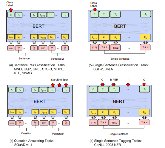
Image taken from BERT paper

In the above figure, we can see that how BERT can be used for different tasks. Among those tasks, (a) and (b) are sequence-level tasks (e.g. spam classification) while (c) and (d) are token-level tasks (e.g. Name Entity Recognition).
Also E represents the input embeddings, Ti represents the contextual representation of token i (also called as a word embeddings), [CLS] is the special token which is useful for sequence level classification task, and [SEP] is the special token to separate two input sentences.

BERT: Feature Extraction

Fine-tuning is not only the way to use the pre-trained BERT model, and guess what? we can use the pre-trained BERT model for creating contextualized word embeddings. The generated contextualized word embeddings by feeding input text to the BERT model can then be used to your existing model to achieve several tasks such as Named Entity Recognition, Question and Answering, etc. The general figure for this process is shown below:

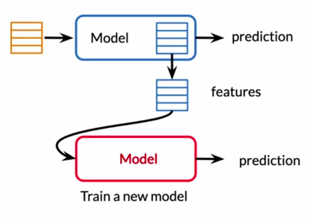
Image taken from NLP specialization

Now, let’s take a look at the context of pretrained BERTbase(stacked 12 transformer encoder) model as an example:

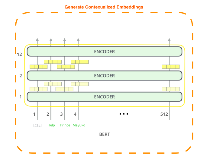
Image taken from the illustrated BERT

From the above figure, we can see that contextualized embeddings for each word in the input sentence are generated by the BERTbase model. As the BERTbase model consists of 12 transformer encoders, so each encoder layer generates contextualized embeddings for each word which it then passes to the upper transformer encoder. So we have 12 choices of contextualized word embeddings which are generated by 12 transformer encoders.

Which encoder layer contextualized word embeddings to use?

• For this BERT paper examines performance between two approaches i.e. Fine-tuning and Feature extraction by applying BERT to the CONLL-2003 Named Entity Recognition task and came to the following conclusion: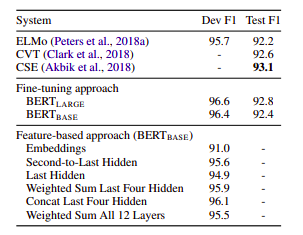
• 
• From above comparison we can see that, result of concatenating last four hidden layer contextualized embedding (Dev F1-score: 96.1) is very close to that of fine-tuning approach (Dev F1-score: 96.4).
• So in this case, we can say that concatenating the output of the last four encoder layers is the best way to use contextualized word embeddings.

Coming this far, you may be wondering we have already an option of fine-tuning the BERT model then why bother to use contextualized embeddings? and one of the several reasons is, there are major computational benefits to pre-compute an expensive representation of the training data once and then run many experiments with cheaper models on top of this representation.

Beyond BERT

There are many other architectures that are improved versions of BERT. All of the improved versions are based on the famous transformer architecture. The improvement is based on Number of layers, Size of datasets, Computation Power, Training method (e.g. NSP, MLM, No NSP, Knowledge Distillation). Some of the most interesting improved versions are RoBERTa, XLnet, DistilBERT, and Many more. Basically, RoBERTa and XLnet improve on the performance whereas DistilBERT improves on the inference speed. The comparison table is shown below:

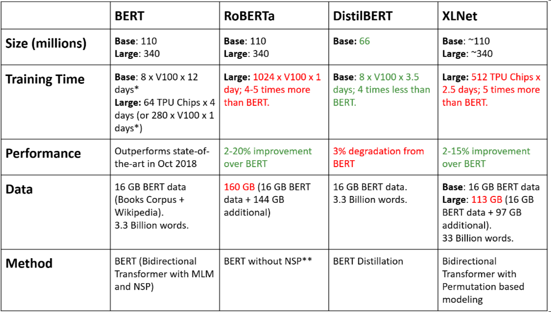
Image taken from BERT, RoBERTa, DistilBERT, XLNet — which one to use?

If you are interested in the roadmap of different models, please have a look at State-of-the-Art NLP models roadmap

References

1. https://mccormickml.com/2019/05/14/BERT-word-embeddings-tutorial/#2-input-formatting
2. https://arxiv.org/pdf/1810.04805.pdf
3. https://github.com/google-research/bert
4. https://jalammar.github.io/illustrated-bert/
5. https://huggingface.co/bert-base-uncased
6. https://towardsdatascience.com/bert-roberta-distilbert-xlnet-which-one-to-use-3d5ab82ba5f8#e18a-828e5fc317c7
7. https://towardsdatascience.com/bert-technology-introduced-in-3-minutes-2c2f9968268c
8. https://machinelearningmastery.com/transfer-learning-for-deep-learning/