

Orthogonal matrices and Gram-Schmidt
In this post we’ll familiarize ourselves with the concepts of projection; projection onto any line, plane and subspace, and we will also discuss about orthogonal vectors, orthogonality of subspaces and why we want to achieve orthogonality. Let’s do a quick recap of the dot product, the dot product gives us a very nice method for determining if two vectors are orthogonal.
The dot product measures angles between vectors by summing the products of the corresponding entries. The dot product of two vectors $x,y$ in $R^{n}$ is
\[x.y=\begin{bmatrix} x_{1}\\ .\\ .\\ .\\ x_{n} \end{bmatrix}.\begin{bmatrix} y_{1}\\ .\\ .\\ .\\ y_{n} \end{bmatrix}=x_{1}y_{1}+...+x_{n}y_{n}\]Dot product of a vector with itself is an important special case. For any vector $x$, we have
- $x.x\geq 0$
- $x.x=0:\Leftrightarrow x=0$
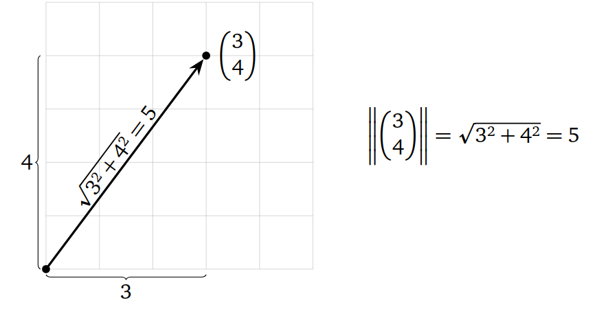
- The length of a vector $x$ in $R^{n}$ is the number
And we can see this is true for vectors in $R^{2}$ from the Pythagorean theorem
This isnt always true, its true only when two vectors are perpendicular. Two vectors $x,y$ in $R^{n}$ are orthogonal or perpendicular if $x.y= 0$ and this is how the dot product define orthogonality. If any of these vectors is a zero vector, they are still orthgonal because zero vector is orthogonal to every vector in $R^{n}$.
Orthogonality of four subspaces
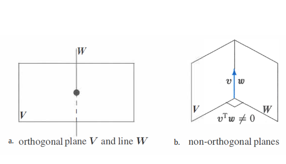
Subspace $V$ is orthogonal to subspace $W$ means: Every vector in $V$ is orthogonal to every vector in $W$ and the two subspaces only intersect at the origin. Orthogonal subspaces $v^{T}w = 0$ for all $v$ in $V$ and all $w$ in $W$. Refer to figure (a) below.
-
Two planes in R3 can’t be orthogonal to each other. If we consider adjacent walls in a room which represent two planes in R3 (figure b) and they intersect at a line rather than the origin. Hence two planes in R3 can’t be orthogonal.
-
The row space is perpendicular to the null space. Every row of $A$ is perpendicular to every solution of $Ax = 0$.
$x$ is orthogonal to each separate rows of $A$ and to the linear combinations of rows of $A$.
-
The column space is perpendicular to the nullspace of $A^{T}$.
-
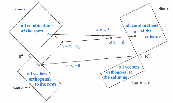
PART 1 of Fundamental Theorem of Linear Algebra: The row and column spaces have the same dimension $r$. The two nullspaces have the remaining dimensions $n-r$ and $m-r$.
-
PART 2 of Fundamental Theorem of Linear Algebra: Perpendicularity of subspaces.
Above stated parts of fundamental theorem of Linear Algebra tells us that the fundamental subspaces are more than just orthogonal, they are orthogonal complements. The orthogonal complement of a subspace $V$ contains every vector that is perpendicular to $V$. This orthogonal subspace is denoted by $V^\perp$ (pronounced “V perp”). By this definition, the nullspace is the orthogonal complement of the row space and the reverse is also true.
The point of complements is that every $x$ can be split into a row space component $X_{r}$ and a nullspace component $x_{n}$ . When $A$ multiplies $x = x_{n} + x_{r}$. Figure below shows what happens to $Ax= Ax_{r} + Ax_{n}$:
Facts about Orthogonal Complements. Let $W$ be a subspace of $R^{n}$ Then:
- $W^\perp$ is also a subspace of $R^{n}$
- $(W^\perp)^\perp = W$
- dim($W^\perp$) + dim($W$) = $n$
There is an $r\;by\;r$ invertible matrix hiding inside $A$, if we throw away the two nullspaces from the row space to the column space, $A$ is invertible.
Projection
Projection Onto a Line
Our goal here is to find projection $p$ and the projection matrix $P$ onto any n-dimensional subspace. Every subspace of $R^{m}$ has its own $m \times m$ projection matrix. So projection onto any subspace is same as projecting onto the column space of $A$, where $A$ is a matrix with basis vectors in its columns.
What we do here is project any vector $b$ onto the column space of any $m \times n$ matrix. For ease we are going to consider 1-dimension example i.e. line, so matrix $A$ will have only one column which is $a$.
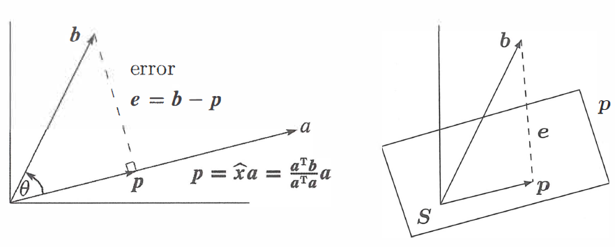
In the figure, a line goes through the origin in the direction of $a$. Along that line, we want the point $p$ closest to $b$. Geometry tells us that we can find this closest point by dropping a perpendicular line (dotted line) from $b$ to the space($a$). That closest and best point $p$ is actually the projection of $b$ onto the line. In another words, when $b$ is projected onto a line, its projection $p$ is the part of $b$ along that line. $p$ is some linear combination of $a$, say $p=\hat{x}a$. So we need to find the $\hat{x}$ that minimizes the distance between $b$ and $\hat{x}$. So we can write in the form of equation below:
\[p = \hat{x}a\] \[a^{T}\left ( b-\hat{x}a \right ) = 0\] \[\hat{x}a^{T}a = a^{T}b\] \[\hat{x}=\frac{a^{T}b}{a^{T}a}\]The projection of $b$ onto the line through $a$ is the vector $p$
\[p = a\frac{a^{T}b}{a^{T}a}\]And the projection matrix $P$:
\[P = \frac{aa^{T}}{a^{T}a}\]Special case 1: If $b = a$ then $\hat{x} = 1$. The projection of $a$ onto $a$ is itself. $Pa= a$.
Special case 2: If $b$ is perpendicular to $a$ then $a^{T}b = 0$. The projection is $p = 0$.
- When $b$ becomes $2b$, projection $p$ becomes $2p$.
- When $a$ becomes $2a$ projection remains same because the projection is being carried out by the same matrix matrix $P$.
Key properties of Projection matrix
-
$P^{T}=P$, i.e. $P$ is symmetric matrix
-
When we do the projection twice, projection is the same point. $P^{2}=P$
Projection Onto a Subspace
Why we do this projection?
Because some system of linear equations $Ax = b$ may not have solution, i.e. when $b$ is not in the column space of $A$. We cant solve this system but we can solve closest problem, so we will solve for $A\hat{x} = p$ instead, where $p$ is the projection of $b$ onto the column space of $A$.
Let us consider we have a plane $S$ in 3D (spanned by vectors $a_{1}$ and $a_{2}$) and a vector $b$ which is not in the plane. What we want to do is project $b$ down onto the plane $S$. The matrix A that describes the plane has two columns $a_{1}$ and $a_{2}$.
- So $p$ is some multiple of $a_{1}$ and $a_{2}$
We want to find the right combination, $\hat{x}$ of the columns of $A$ so that $e$ vector is perpendicular to the plane.
We have,
\[e = b-A\hat{x}\]\(a_{1}^{T}(b-A\hat{x})=0\) \(and\; a_{2}^{T}(b-A\hat{x})=0\)
\[\begin{bmatrix} a_{1}^{T}\\a_{2}^{T} \end{bmatrix}\left (b-A\hat{x}\right )=\begin{bmatrix} 0\\0 \end{bmatrix}\]$A^{T}(b-A\hat{x})=0$, which is similar to the equation $a^{T}(b-\hat{x}a)=0$ in case of 1-D
The combination $p=\hat{x_{1}}a_{1}+…+\hat{x_{n}}a_{n}=A\hat{x}$ that is closest to $b$ comes from $\hat{x}$.
When it is not just 2 but $n$ linearly independent vectors in $R^{m}$, then:
\(A^{T}(b-A\hat{x})=0\) \(or \;A^{T}A\hat{x}=A^{T}b\)
$A^{T}A$ is $n$ by $n$ symmetric matrix. It is invertible if the $a’s$ are independent.
The projection of $b$ onto the subspace is: $p = A\hat{x} = A(A^{T}A)^{-1}A^{T}b$
And the projection matrix is:
$P=A(A^{T}A)^{-1}A^{T}$
- From the equation we know $e$ is in the nullspace of $A^{T}$. This is what the big picture of four fundamental subspaces describes, i.e. column space and nullspace of $A^{T}$ are perpendicular.
Compare with the projection onto a line, when A has only one column: $A^{T}A$ is $a^{T}a$.
For $n=1$ $\hat{x}=\frac{a^{T}b}{a^{T}a}$ and $p=a\frac{a^{T}b}{a^{T}a}$ and $P=\frac{aa^{T}}{a^{T}a}$
- $a^{T}a$ is a number in case of 1-D but in 3-D (or n-D where n>1) we have inverse of matrix $A^{T}A$.
-
If A was square invertible matrix then we could simplify $P$ and get identity matrix $I$. $P = AA^{-1}(A^{T})^{-1}A^{T}$, here everything cancels and we get $I$. But in case of rectangular matrix A, it has no inverse and we cannot split $\left ( A^{T}A \right )^{-1}$ into $A^{-1}$ times $(A^{T})^{-1}$.
- $A^{T}A$ is not always invertible.
Example: We have matrix A,
\[A=\begin{bmatrix}1& 1\\ 1& 2\\ 1& 5\end{bmatrix}\] \[A^{T}A=\begin{bmatrix}1 &1 & 1\\1&2 &5 \end{bmatrix}\begin{bmatrix}1& 1\\ 1& 2\\ 1&5\end{bmatrix}=\begin{bmatrix} 3 & 8\\ 8 & 30 \end{bmatrix}\]- Here $A^{T}A$ is invertible since A has independent columns. We can see beforehand if $A^{T}A$ is invertible from the columns of $A$. $A$ is rank 2 matrix, so is $A^{T}A$. So the product of matrix $A$ won’t have any bigger rank.
Least Squares Approxomations
When there are more linear equations than unknowns i.e., when the system is overdetermined, it is usually impossible to find a solution which satisfies all the equations and we often look for a solution which approximately satisfies all the equations. Suppose that $Ax=b$ does not have a soultion and we try to solve for best approximate solution and the best approximate solution is called the least-squares solution.
Least-Squares Solutions
Let us define what we mean by a “best approximate solution” to an inconsistent equation $Ax=b$.
Let $A$ be an $m*n$ matrix and let $b$ be a vector in $R^{m}$. A least-squares solution of the matrix equation $Ax=b$ is a vector $\hat{x}$ in $R^{n}$ such that \(dist(b,A\hat{x})<=dist(b,Ax)\)
for all other vectors $x$ in $R^{n}$.
We know the distance between two vectors $v$ and $w$ is $dist(v,w)=\left | v-w \right |$. The term “least squares” comes from the fact that $dist(b,Ax)=\left | b-A\hat{x} \right |$ is the square root of the sum of the squares of the entries of the vector $b-A\hat{x}$. So a least-squares solution solves the equation $Ax=b$ as closely as possible, in the sense that the sum of the squares of the difference $b-Ax$ is minimized.
Column space of $A$, $Col(A)$ is the set of all vectors of the form $Ax$. Hence, the closest vector of the form $Ax$ to $b$ is the orthogonal projection of $b$ onto $Col(A)$ denoted by $b_{Col(A)}$.
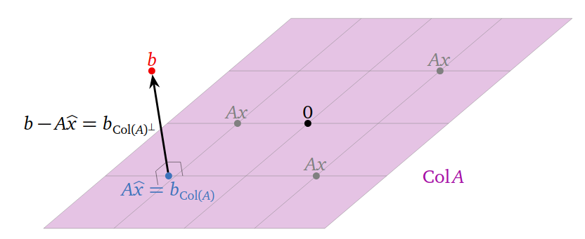
A least-squares solution of $Ax=b$ is a solution $\hat{x}$ of the consistent equation $Ax=b_{Col(A)}$.
Infinitely many least-squares solution:Least-squares solution need not be unique: if the columns of $A$ are linearly dependent, then $Ax=b_{Col(A)}$ has infinitely many solutions.
Orthonormal bases and Gram-Schmidt
This part highlights on why orthogonality is good and how can we achieve it. Using an orthonormal basis or a matrix with orthonormal columns makes calculations much easier. Dot products are zero, so $A^{T}A$ will be diagonal. It becomes easy to find $\hat{x}$ and $p=A\hat{x}$. Gram-Schmidt chooses combinations of the original basis vectors to produce right angles. Those original vectors are the columns of $A$, probably not orthogonal. The orthonormal basis vectors will be the columns of a new matrix $Q$.
Suppose we have a set of vectors $q_{1},q_{2}…,q_{n}$ and it is not just any set of vectors but have some interesting properties.
-
All of these vectors are normalized (have unit length). $\left | q_{i} \right |=1$ for $i=1,2,…,n$ or $\left | q_{i} \right |^{2}=1$ or $q_{i}.q_{i}=1$
-
All of the vectors are orthogonal to each other. The dot product of a vector with itself is 1 and with any other vectors in the set, it is zero .
-
So this set of unit and orthogonal vectors is known as orthonormal set. One fact about orthonormal set is that the vectors are linearly independent.
The vectors $q_{1},q_{2}…,q_{n}$ are orthonormal if \(q_{i}^{T}q_{j}=\left\{\begin{matrix} 0\; when\; i\neq j \; \text{(orthogonal vectors)}\\ 1\; when \;i=j\;\text{(unit vectors)} \end{matrix}\right.\)
Matrices with orthonormal columns are a new class of important matrices besides triangular, diagonal, permutation, symmetric, reduced row echelon, and projection matrices. We call them orthonormal matrices. A square orthonormal matrix $Q$ is called an orthogonal matrix. If $Q$ is square, then $Q^{T}Q=I$ tells us that $Q^{T}=Q^{-1}$.
Orthonormal columns are good
Suppose $Q$ has orthonormal columns. The matrix that projects onto the column space of $Q$ is:
\[P = Q^{T}(Q^{T}Q)^{-1}Q^{T}.\]If the columns of $Q$ are orthonormal, then $Q^{T}Q = I$ and $P = QQ^{T}$. If $Q$ is square, then $P = I$ because the columns of $Q$ span the entire space. Many equations become trivial when using a matrix with orthonormal columns. If our basis is orthonormal, the projection component becomes: \(\hat{x} = q^{T}b\)
Gram-Schmidt
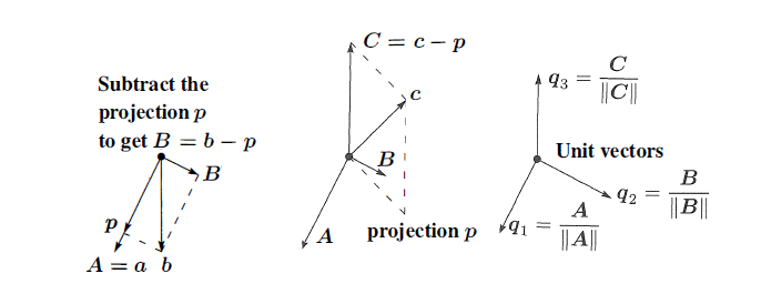
Our goal now is to make the matrix orthonormal. We start with two independent vectors $a$ and $b$ and want to find orthonormal vectors $q_1$ and $q_2$ that span the same plane. We start by finding orthogonal vectors $A$ and $B$ that span the same space as $a$ and $b$. Then the unit vectors $q_{1}=\frac{A}{\left | A \right |}$ and $q_{2}=\frac{B}{\left | B \right |}$ form the desired orthonormal basis.
Let $A = a$. We get a vector orthogonal to $A$ in the space spanned by $a$ and $b$ by projecting $b$ onto $a$ and letting $B = b − p$. ($B$ is what we previously called $e$.)
\[B=b-\frac{A^{T}b}{A^{T}A}A\]If we multiply both sides of this equation by $A^{T}$, we see that $A^{T}B=0$. If we had started with three independent vectors, $a,b$ and $c$, then we would find a vector $C$ orthogonal to both $A$ and $B$ by subtracting from $c$ its components in the $A$ and $B$ directions: \(C=c-\frac{A^{T}c}{A^{T}A}A-\frac{B^{T}c}{B^{T}B}B\)
For example, suppose $a=\begin{bmatrix} 1\ 1\ 1 \end{bmatrix}$ and $b=\begin{bmatrix} 1\ 0\ 2 \end{bmatrix}$ are column vectors. Then $A=a$ and:
\[B=\begin{bmatrix} 1\\ 0\\ 2 \end{bmatrix}-\frac{A^{T}b}{A^{T}A}\begin{bmatrix} 1\\ 1\\ 1 \end{bmatrix}\] \[=\begin{bmatrix} 1\\ 0\\ 2 \end{bmatrix}-\frac{3}{3}\begin{bmatrix} 1\\ 1\\ 1 \end{bmatrix}\] \[=\begin{bmatrix} 0\\ -1\\ 1 \end{bmatrix}\]Normalizing, we get: \(Q=\begin{bmatrix} q_{1} &q_{2} \end{bmatrix}\) \(=\begin{bmatrix} \frac{1}{\sqrt{3}} &0 \\ \frac{1}{\sqrt{3}} & \frac{-1}{\sqrt{2}}\\ \frac{1}{\sqrt{3}} & \frac{1}{\sqrt{2}} \end{bmatrix}\)
The column space of $Q$ is the plane spanned by $a$ and $b$. The equation $A=QR$ relates to our starting matrix $A$ to the result $Q$ of the Gram-Schmidt process, where $R$ is upper triangular matrix.
Suppose $A=\begin{bmatrix}a_{1} & a_{2} \end{bmatrix}$. Then:
\[A = QR\] \[\begin{bmatrix} a_{1} & a_{2} \end{bmatrix}=\begin{bmatrix} q_{1} & q_{2} \end{bmatrix}\begin{bmatrix} a^{T}_{1}q_{1} & a^{T}_{2}q_{1} \\ a^{T}_{1}q_{2} & a^{T}_{2}q_{2} \end{bmatrix}\]References